Unsupervised Learning
In a supervised learning procedure, the machine tries to learn the underlying relationships between a set of example inputs and their corresponding outputs.
In an unsupervised learning procedure, the machine only tries to learn about the internal structure of the input examples.
This allows us to extract meaningful features and patterns from the input data.
Unsupervised learning is useful in various forms of data analysis and dimensionality reduction.
Unsupervised learning can also be applied to generative or creative applications. For example, we could learn about the kinds of patterns that exist within a particular composer's work and then use this to generate new compositions in the style of that artist.
It can also be useful in improving the quality of a supervised learning procedure. This is particularly true in cases where we have far more input examples than we have correctly labeled corresponding outputs. For example, the internet provides an endless supply of images from which we could learn internal patterns. But only a small portion of these images come with reliable descriptions of the images' contents. Unsupervised learning allows us to learn common patterns across both labeled and unlabeled images and then use these underlying patterns to associate previously unlabeled images with labels that correspond to structurally similar images.
This approach bears some resemblance to our own learning process in the sense that we have many experiences interacting with a particular kind of object, but a much smaller number of experiences in which another person explicitly tells us the name of that object.
Unsupervised learning in general and in its relation to supervised learning can tell us a lot about the nature of thought and the representation of ideas.
Restricted Boltzmann Machine Architecture
Conceptual Overview
Based on my article Machine Learning and Improvisation.
A Restricted Boltzmann Machine (RBM) is a two-layer neural network composed of a visible layer and a hidden layer.
Each unit in the visible layer is connected to each unit in the hidden layer. The visible units are not connected to one another and the hidden units are not connected to one another.
An RBM observes real-world patterns and tries to create a lower-dimensional representation of those patterns.
We can also stack multiple RBMs on top of one another to reduce the dimensionality of the patterns even further. One common architecture for stacked RBMs is called a Deep Belief Network (DBN).
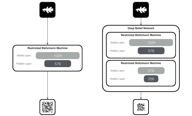
The goal of the training process is to produce lower dimensional representations that can then be used to “reconstruct” approximations of the original inputs.
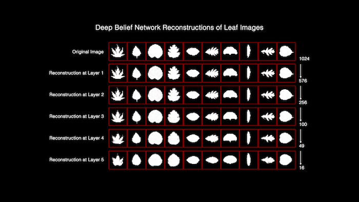
In the animation below, we will train a DBN on leaf images from 100 species, using 16 images per species.
You can think of this as a kind of compression algorithm, improvised in relation to the neural network’s experience.
The network compresses information by finding component patterns across many input examples. It can then use these component patterns as building blocks to describe the whole.
This is an efficient way to store information because it means we don’t need to hold onto every detail of every input example. We can use a more general vocabulary derived from all of the examples to describe each particular example.
The reconstruction of an input example through this process is not exact. But that’s what’s interesting about it!
Notice how the approximation changes as we go to deeper layers of the neural network:
And notice what happens when we reconstruct partially obfuscated images:
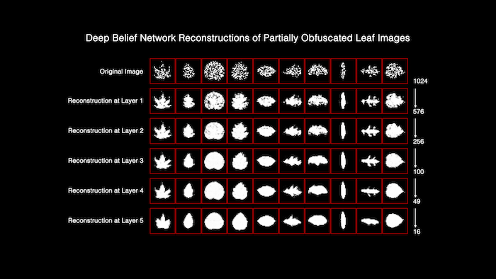
This is somewhat like our minds filling in the missing pieces of a face that has been partially occluded by some other object such as a telephone pole.
Representing experiences through a shared set of component patterns means that we don’t have to treat each as entirely separate from or incomparable to each other. We can fill gaps in our experiences by borrowing from our memory of other similar experiences.
Tracing the Path of a Single Input
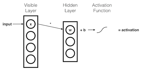
The \(x\) component is multiplied by a \(weight\) and added to a \(bias\). The result of this operation is then passed through an activation function.
The resulting \(activation\) represents the strength of the signal passing through the hidden node, given input \(x\).
More generally:
\( activation = activationFunction( weight * input + hiddenBias ) \)
Combining Weighted Inputs
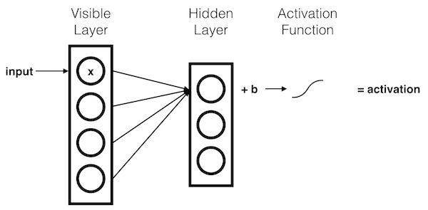
Each \(x\) component is multiplied by a separate \(weight\). These products are summed together and added to a \(bias\). The result of this operation is passed through an activation function.
Multiple Inputs
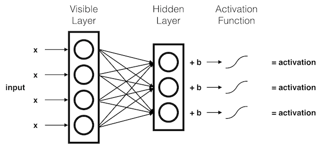
Each hidden node receives the components of the input signal, multiplied by their corresponding \(weights\). These products are summed together and added to the hidden node's \(bias\). The results of these operations are passed through an activation function.
Reconstruction
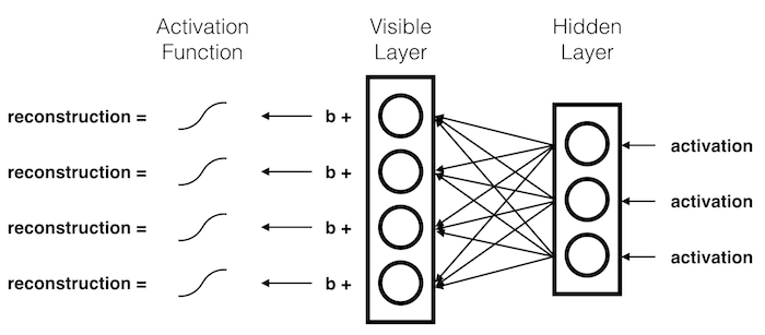
During reconstruction, the hidden activations are passed backward through the network.
The \(activations\) are multiplied by their corresponding \(weights\). These products are summed together and added to the visible node's \(bias\). The results of these operations are passed through an activation function.
More generally:
\( reconstruction = activationFunction( {activation}^{T} * weight + visibleBias ) \)
The output of this reconstruction process acts as an approximation of the original input.
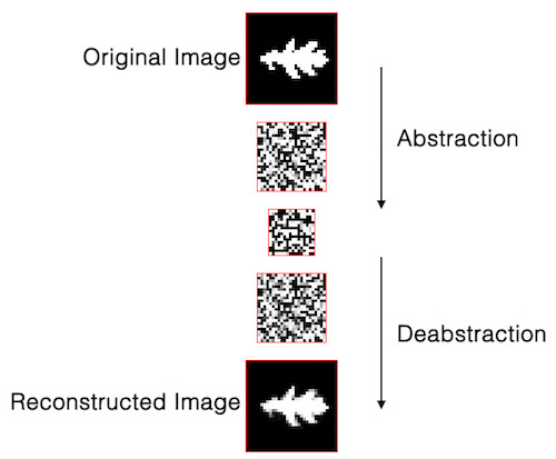
Abstraction and Deabstraction
The forward and backward passes described above give us two symmetrical processes for abstracting and deabstracting (or, compressing and decompressing) information:
Get Hidden Activations (Propagate Up)
\( activationsH = \frac{1}{1 + {e}^{-(inputV \cdot weights + biasH)}} \\ \)
Get Visible Activations (Propagate Down)
\( activationsV = \frac{1}{1 + {e}^{-(inputH \cdot {weights}^{T} + biasV)}} \\ \)
Training Restricted Boltzmann Machines
Based on CSC321: Neural Networks, by Geoffrey Hinton.
An Inefficient Approach
Learning Rule
\( \Delta{{W}_{ij}} = learningRate * ( {\langle{v}_{i}{h}_{j}\rangle}^{0} - {\langle{v}_{i}{h}_{j}\rangle}^{\infty} ) \)
Learning Procedure
- Apply a training example to the visible units
- Alternate between:
- Updating all hidden units in parallel
- Updating all visible units in parallel
- After many alternations (timestep \(\infty\)), the system will reach thermal equilibrium.
- We can now measure the correlation between \(v_i\) and \(h_j\).
Limitations
- We have to perform this alternation many times before it reaches thermal equilibrium.
- If we don't perform it a sufficient number of times, the learning may go wrong.
- But, it turns out that we can take a shortcut: Contrastive Divergence.
Contrastive Divergence
Learning Rule
\( \Delta{{W}_{ij}} = learningRate * ( {\langle{v}_{i}{h}_{j}\rangle}^{0} - {\langle{v}_{i}{h}_{j}\rangle}^{1} ) \)
Learning Procedure
- Apply a training example to the visible units
- Update all hidden units in parallel
- Update all visible units in parallel
- Update all hidden units again
Instead of waiting for thermal equilibrium, we use the measurements produced by one update step.
Why Contrastive Divergence Works
- If we start from the data, the Markov chain will wander away from the data values themselves and towards values it likes more (an equilibrium distribution).
- After only a few steps, we can see what direction it is wandering in.
- Since we know the initial weights are bad, it is wasteful to let them go all the way to equilibrium. We know how to change the weights to stop them from wandering away from the data without going all the way to equilibrium.
- We simply need to lower the probability of the reconstructions it produces after one full step and then raise the probability of the data.
- This will stop the chain from wandering away from the data.
- The learning will cancel out once the reconstructions and the data have the same distribution as one another.
Implementing a Restricted Boltzmann Machine
import numpy as np

def sigmoid(x):
    '''sigmoid function'''
    return 1.0 / ( 1.0 + np.exp( -x ) )

class Rbm:
    def __init__(self, name, sizeV, sizeH, continuous = False):
        self.name    = name
        self.is_crbm = continuous
        # Initialize weights:
        self.weights = np.array( np.random.uniform( -1.0 / sizeV, 1.0 / sizeV, ( sizeV, sizeH ) ) )
        # Initialize biases:
        self.biasH   = np.zeros( sizeH )
        self.biasV   = np.zeros( sizeV )

    def getErrorRate(self, samples, reconstructions):
        '''returns mean square error'''
        return np.mean( np.square( samples - reconstructions ) )

    def trainEpoch(self, training_samples, learn_rate, cd_steps, batch_size):
        error      = 0.0
        num_rows   = training_samples.shape[ 0 ]
        # Iterate over each training batch:
        for bstart in range( 0, num_rows, batch_size ):
            # Compute batch stop index:
            bstop = min( bstart + batch_size, num_rows )
            # Compute batch size:
            bsize = bstop - bstart
            # Compute batch multiplier:
            bmult = learn_rate * ( 1.0 / float( bsize ) )
            # Slice data:
            bsamples = training_samples[ bstart:bstop, : ]
            # Get hidden activations and samples:
            aH_0, sH_0 = self.getHiddenSample( bsamples )
            # Perform each contrastive divergence step:
            for i in range( cd_steps ):
                aV_inf, sV_inf, aH_inf, sH_inf = self.getGibbsHvh( ( sH_0 if i == 0 else sH_inf ) )
            # Update weights:
            self.weights += bmult * ( np.dot( bsamples.T, aH_0 ) - np.dot( sV_inf.T, aH_inf ) )
            # Update biases:
            self.biasV   += bmult * np.mean( bsamples - sV_inf, axis = 0 )
            self.biasH   += bmult * np.mean( aH_0 - aH_inf, axis = 0 )
            # Scale batch error and accumulate total:
            error += self.getErrorRate( bsamples, sV_inf ) * ( float( bsize ) / float( num_rows ) )
        # Return training error:
        return error

    def train(self, training_samples, validation_samples, learn_rate, cd_steps, epochs, batch_size = 10, report_freq = 10, report_buff = 100):
        # Perform each training epoch:
        for epoch in range( epochs ):
            training_error = self.trainEpoch( training_samples, learn_rate, cd_steps, batch_size )
            # Report error, if applicable:
            if ( epoch + 1 ) % report_freq == 0:
                # Compute validation error:
                val_aH, val_sH, val_aV, val_sV = self.getGibbsVhv( validation_samples )
                validation_error = self.getErrorRate( validation_samples, val_sV )

    def getHiddenActivations(self, inputV):
        return sigmoid( np.dot( inputV, self.weights ) + self.biasH )

    def getVisibleActivations(self, inputH):
        return sigmoid( np.dot( inputH, self.weights.T ) + self.biasV )

    def getHiddenSample(self, inputV, force_binomial = False):
        aH = self.getHiddenActivations( inputV )
        return [ aH, self.getSample( aH ) if ( force_binomial or not self.is_crbm ) else aH ]

    def getVisibleSample(self, inputH, force_binomial = False):
        aV = self.getVisibleActivations( inputH )
        return [ aV, self.getSample( aV ) if ( force_binomial or not self.is_crbm ) else aV ]

    def getGibbsHvh(self, inputH, force_binomial = False):
        aV, sV = self.getVisibleSample( inputH, force_binomial )
        aH, sH = self.getHiddenSample( sV, force_binomial )
        return [ aV, sV, aH, sH ]

    def getGibbsVhv(self, inputV, force_binomial = False):
        aH, sH = self.getHiddenSample( inputV, force_binomial )
        aV, sV = self.getVisibleSample( sH, force_binomial )
        return [ aH, sH, aV, sV ]

    @staticmethod
    def getSample(activations):
        return np.random.binomial( 1, activations, activations.shape )
Take a look at the full Restricted Boltzmann Machine example code.
Getting Started with Docker and LaunchBot
Next week, we will be using Google’s TensorFlow library.
To prepare for that, I would like to spend a bit of time at the end of class installing Docker and LaunchBot, two tools that will help us to streamline our TensorFlow work.
Please see the LaunchBot Getting Started Tutorial for instructions on how to install Docker and LaunchBot.
Homework
Assignment
- Please see The Great Hyperparameter Hunt for this week's assignment.
Readings