What is Deep Learning?
From Alan Turing onwards, the history of machine learning has been marked by alternating periods of optimism and discouragement over the field’s prospects for applying its conceptual advancements to practical systems and, in particular, to the construction of a general-purpose artificial intelligence.
These periods of discouragement, which are often called AI winters, have generally stemmed from the realization that a particular conceptual model could not be easily scaled from simple test problems to more complex tasks.
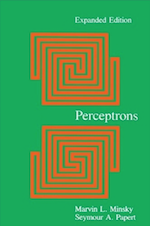
This occurred in the 1960s when Marvin Minsky and Seymour Papert conclusively demonstrated that perceptrons could not solve what are called linearly inseparable problems.
In the late 1980s, there was some initial excitement over the backpropagation algorithm’s ability to overcome this issue. But another AI winter occurred when it became clear that the algorithm’s theoretical capabilities were practically constrained by computationally intensive training processes and the limited hardware of the time.
Over the last decade, a series of technical advances in the architecture and training procedures associated with artificial neural networks, along with rapid progress in computing hardware, have contributed to a renewed optimism for the prospects of machine learning.
One of the central ideas driving these advances is the realization that complex patterns can be understood as hierarchical phenomena in which simple patterns are used to form the building blocks for the description of more complex ones, which can in turn be used to describe even more complex ones.
The systems that have arisen from this research are referred to as deep because they generally involve multiple layers of learning systems which are tasked with discovering increasingly abstract or high-level patterns. This approach is often referred to as hierarchical feature learning.
Learning about a complex idea from raw data is challenging because of the immense variability and noise that may exist within the data samples representing a particular concept or object.
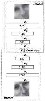
Rather than trying to correlate raw pixel information with the notion of a human face, we can break the problem down into several successive stages of conceptual abstraction.
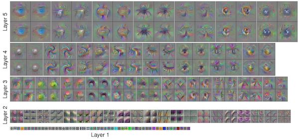
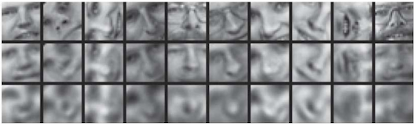
In the first layer, we might try to discover simple patterns in the relationships between individual pixels. These patterns would describe basic geometric components such as lines.
In the next layer, these basic patterns could be used to represent the underlying components of more complex geometric features such as surfaces, which could be used by yet another layer to describe the complex set of shapes that compose an object like a human face.
This approach allows machine learning researchers to tackle incredibly complex learning problems and has led to a renaissance period in the field.
Building Intuition for Machine Learning Problems
As you begin to work with machine learning, one of the most important things you can do is to start developing an intuition for what kinds of problems are well-suited to a machine learning solution.
The key component to this is being able to think through how to teach a machine about a particular concept from a set of examples or experiences.
Machine learning systems are, of course, much less complex and capable than the human mind. But like us, they are experiential learners. Therefore, we must act as their teachers.
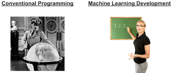
Writing conventional code is much more like being a dictator. As a programmer, you dictate a concrete series of actions that the machine should perform. This is a much more straightforward process than teaching.
As a first step in assessing whether a problem is well-suited to machine learning, you should always ask yourself, "Can I articulate a concrete series of actions that would produce the desired functionality?"
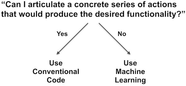
If the answer is yes, then you should use a conventional programmatic approach rather than a machine learning one. If the problem seems too complex or nebulous to be described by a concrete procedure, but you can imagine a set of example experiences that embody the concept, then machine learning may be the ideal solution.
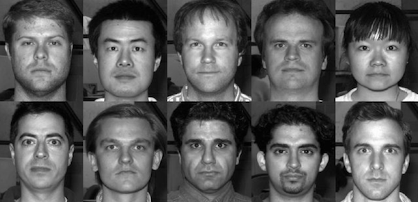
As humans, we draw upon years of prior experience in solving complex problems. We do this so intuitively, that it can be very difficult to think about how we actually do this. Recognizing a face, for instance, is a very complex task. But we’ve done it so many times, it feels completely automatic. How did we learn to do it?
For a task like facial recognition, it may be the case that some aspects of this capability have been baked into our neural architecture through our evolutionary development. But, we’ll leave that aside.
For the most part, we have learned to recognize faces by observing them and by correlating those experiences with other contextual information. In other words, when you were a child, someone probably pointed across the room and asked you, "Do you see that person? Who is that?"
An experience like this helped you to correlate the visual appearance of a person with the word person. Repeated many times and in many different contexts, experiences of this kind led you to a robust and intuitive capability to identify other humans.
Your parents and teachers could not dictate what ideas your mind should contain. They could only provide you with experiences that would lead you to synthesize those ideas for yourself.
There are many different machine learning algorithms and each comes with its own strengths, weaknesses and technical details. But those details can come later.
The starting point is to get a feel for how to demonstrate a concept through a set of examples.
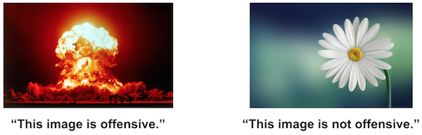
It may be helpful to begin by asking yourself how you would demonstrate the concept to another person. For example, if you were trying to teach a person to distinguish between offensive and inoffensive images you could gather a large collection of images, show each image to the other person and say "I find this image offensive" or "I do not find this image offensive."
Remember that, generally speaking, a machine learning system is starting with no prior experience of the world and cannot draw upon other high level concepts it already knows.
Therefore, you cannot teach it to recognize offensive images by saying to it "any image that contains violence is offensive." The machine doesn’t know what violence means, so this term will not help it to learn the meaning of offensive.
The machine must instead learn to recognize patterns within the pixels that comprise images and then correlate these patterns with labels such as offensive or inoffensive.
Yet, distinctions such as offensive and inoffensive are not objective in nature.
If we asked a group of people to classify a series of images in these terms, we would be likely to give somewhat different answers from each person. In this sense, the quality of our machine learning system is, above all else, dependent upon the nature of the data or experiences we train it on.
If we trained the machine only on my opinion of whether an image was offensive, others might not agree with the predictions made by this system. This does not necessarily mean that the system is broken. It simply means that the system has been trained to do something different from what the user expects. In truth, the system was not trained to identify offensive images. It was been trained to recognize what I would call offensive images. We might call this a perfectly functioning system, so long as I am its only user.
But, if we define a perfectly functioning system as one whose predictions approximate the average citizen, then we should ask a large number of people whether each image is offensive and use the majority opinion as the label we present to the machine.
That is to say, if we want to change the system’s behavior or outputs, we have to change the experiences we use to teach it.
As we dive deeper into specific applications of machine learning, we will need to address other important issues such as determining whether a specific problem would be best addressed by supervised, unsupervised, semi-supervised or reinforcement learning.
In these deeper questions, too, if will often be helpful to start by carefully thinking through what kinds of experiences or examples can be used to convey the concept or behavior we wish the machine to learn.
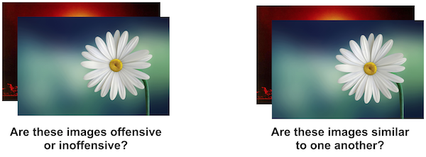
We may wish to have the machine learn to identify an offensive image by showing it example images and telling it whether the image is offensive or inoffensive. This sounds like a supervised learning problem in which machine will try to find correlations between a set of example inputs and their corresponding outputs.
We may instead wish to show the machine a bunch of images and ask it to figure out which photos are similar to one another. This sounds like an unsupervised learning problem because we have not specified how the concept of similarity would be explicitly demonstrated through the data, therefore implying that the machine should make this determination through its own observations.
There are many details to choosing and working with a machine learning algorithm. But, being able to clearly articulate a learning problem will make it significantly easier to evaluate whether a particular learning algorithm is well-suited to your objective.
A Brief Tour of Graph Theory
In 1736, the mathematician Leonhard Euler published a paper on the Seven Bridges of Königsberg, which addressed the following question:
Königsberg is divided into four parts by the river Pregel, and connected by seven bridges. Is it possible to tour Königsberg along a path that crosses every bridge once, and at most once? You can start and finish wherever you want, not necessarily in the same place.
Euler looked at this problem from the perspective of how the edges, vertices and faces of a convex polyhedron relate to one another and in the process gave rise to a new study within mathematics, now called graph theory.
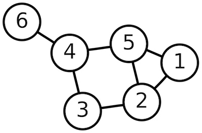
More generally, graph theory is the study of mathematical structures that can be used to model the pairwise relationships between objects. Graphs are comprised of vertices, which are connected to one another by edges.
In a directed graph, an edge represents a uni-directional relationship: a connection that flows from Vertex A to Vertex B, but not from Vertex B to Vertex A. In an undirected graph, an edge represents a bi-directional relationship: the connection flows from A to B as well as from B to A.
In a cyclic graph, the connections between vertices can form loops whereas in an acyclic graph they cannot.
These distinctions as well as others made by graph theory can be used to model an astoundingly wide variety of systems. It is used in physics, chemistry, biology, linguistics and many other fields. It is especially relevant to the field of computer science. Computer programs can be thought of as graphs that describe a flow of information through a series of operations. 2D and 3D design tools often represent users' projects as scenegraphs, which describe the hierarchical relationships between a series of geometric components.
Artificial neural networks are often thought about in these terms as well. Some neural architectures, such as many forms of classifiers, can be seen as directed acyclic graphs. Others, such as many forms of auto-encoders, can be represented as undirected graphs in which unencoded information can be passed in one direction to encode it while encoded information can be passed in the other direction to decode it. Recurrent neural networks are ones that allow loops (or "cycles") in their flow of information.
Machine learning draws upon metaphors from many other fields including neuroscience and thermodynamics. But graph theory has proven to provide a particularly good vocabulary for describing the kinds of nodal relationships that comprise the various forms of neural network models. Google's open-source machine learning library TensorFlow uses this mentality as its central organizing principle, as do several other popular machine learning toolkits. The "flow" in "TensorFlow" is a reference to the flow of information through a graph.
Though graph theory is a complex study in its own right, familiarity with its basic distinctions can be useful in understanding the composition of artificial neural networks.
Additional Resources
Perceptrons
History
- Perceptron algorithm invented by Frank Rosenblatt in 1957.
- Rosenblatt developed the algorithm for the US Office of Naval Research for image recognition purposes.
- Rosenblatt made bold claims about the future of Artificial Intelligence and the ability to teach machines to walk, talk, see, etc. This led to controversy.
- In 1969, Marvin Minsky and Seymour Papert published the book, Perceptrons, which conclusively showed that it was impossible for perceptrons to learn an exclusive-or (XOR) function.
- Minsky and Papert were aware that using multiple layers in the network would allow the representation of an XOR function. But the common misunderstanding of an artificial neural network's limitations led to a stark decline in interest and funding - an AI Winter.
- In the 1980s, interest grew again with work on Multilayer Perceptrons and the Backpropagation algorithm, developed by David Rumelhart, Geoff Hinton, et al.
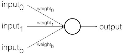
Basic Model
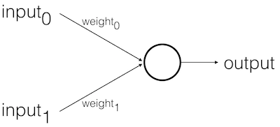
Feed Forward Stages
- Receive inputs
- Weigh inputs
- Sum inputs
- Generate output
Example
- \(input_0\) = 12
\(input_1\) = 4 - (weights are initially random)
\(weight_0\) = 0.5
\(weight_1\) = -1.0
\(input_0 * weight_0\) = 12 * 0.5 = 6
\(input_1 * weight_1\) = 4 * -1.0 = -4 - \(sum\) = 6 + -4 = 2
- \(output\) = Sign( \(sum\) ) = Sign( 2 ) = +1
The Perceptron Algorithm
- For every input, multiply that input by its weight.
- Sum all of the weighted inputs.
- Compute the output based on that sum passed through an activation function.
Here, the activation function will be the sign of the sum.
Electrical Analogy
An electronic logic gate is a lot like a pre-trained Perceptron.
Consider Alan Turing's comment in Intelligent Machinery:
"Many unorganized machines have configurations such that if once that configuration is reached, and if the interference thereafter is appropriately restricted, the machine behaves as one organized for some definite purpose." (p14-15)
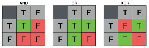
Here are the truth tables for two common logic gates:
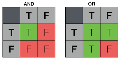
How could we implement these logical operations in electronic components?
AND Gate:

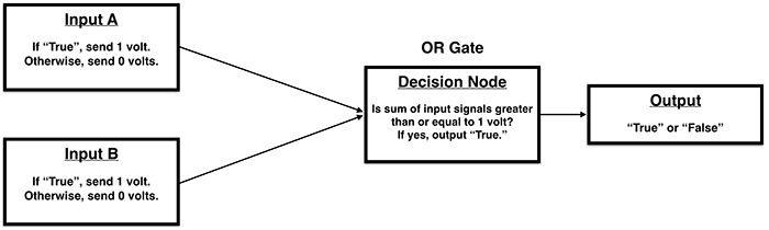
OR Gate:
Biological Analogy
Biological neurons fire when there is sufficient activity in their inputs.
Loosely, we might think of this as:
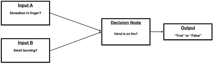
Of course, biological networks are complex (multilayered, so to speak).
The human brain definitely does not contain a single neuron that addresses the question of whether our hand is on fire.
In a more general (but still very loose) sense, it may be reasonable to say that we:
- monitor a group of input sensors
- weigh their relative importance
- determine the most appropriate behavior in response to these inputs
(Prelude to) Training Perceptrons
So far, we've looked at the feed-forward behavior of the Perceptron. But we have not yet considered how we train it to perform this behavior. In the above logic gate examples, how did we determine the proper signal voltages for each input? For these simple examples, we knew the desired behaviors and could therefore design for them explicitly. For more complex problems, however, it would be far more difficult to do so. Ideally, we would like the machine to implement the desired behavior on its own by learning from the examples that have been shown to it.
Biases
Before we look more closely at the training process, let's consider a possible difficulty:
Recall the following step in the feed-forward process:
\(input_0 * weight_0\)
\(input_1 * weight_1\)
Given this, what would happen if:
\(input_0\) = 0
\(input_1\) = 0
In this case, it doesn't matter what the weights are!
The sum will always be zero.
To avoid this problem, we generally add an extra input to our Perceptron, called the bias input.
The bias input always has a value of 1 and is also weighted.
\(input_0\) = 0
\(input_1\) = 0
\(input_b\) = 1
\(input_0 * weight_0\) = 0
\(input_1 * weight_1\) = 0
\(input_b * weight_b\) = \(weight_b\)
In this case, the bias alone determines the output.
It biases the Perceptron's understanding of the line's position relative to the point [ 0, 0 ].
Implementation Detail
You could implement biases in a few different ways:
- In your dataset ([ 1, -1 ] becomes [ 1, -1, 1 ], e.g.)
- This option is most undesirable because it requires manually editing your dataset.
- When you run the Perceptron, you could append a 1 to the end of each input vector
- This option is ok for small vectors, but is ultimately inefficient because it generally requires reallocating / copying lots of arrays.
- Store bias separate from other weights and add it in during the summing step.
- This option is favorable and standard in many implementations.
Supervised Training Procedure
We train the Perceptron by showing it examples for which we know the expected output, adjusting weights according to the incorrectness of the Perceptron's guessed output.
The Procedure
- Provide the Perceptron with inputs for which there are known outputs.
- Ask the Perceptron to guess the outputs.
- Compute the error.
- Adjust all weights according to error.
- Return to Step 1 and repeat.
Error Definition
\( Error = {Output}_{Expected} - {Output}_{Guessed} \)
Error Delta
\( \Delta{Weight} = Error * Input \)
Weight Update
\( {Weight}_{New} = {Weight}_{Old} + \Delta{Weight} \)
Learning Rate
We generally don't want to learn too much too quickly (from any one example).
So, we use a learning constant to limit the impact of our weight change:
\( {Weight}_{New} = {Weight}_{Old} + \Delta{Weight} * LearningConstant \)
where \(LearningConstant\) is a scalar value (presumably \(\lt\) 1).
Finding a good learning constant is relative to the dataset.
Experimentation is the best first approach, though it's possible to be more systematic.
We'll discuss this and related issues more in subsequent weeks.
Limitations of the Perceptron Model
Unfortunately, Perceptrons are very limited in their learning capabilities. To better understand these limitations, let's consider a third form of logic gate: exclusive-or (XOR).
The behavior of an XOR gate could be worded as:
"The output will be activated if one or the other of the inputs is active, but not if both inputs are active."
Go back to the earlier electrical diagrams for AND and OR and see whether you can find input signal voltages that will enable the behavior of an XOR gate.
Start with the OR gate:
Again, we set the activation threshold to 1 volt and each of the input signals to 1 volt.
If only one of the inputs is active, then the sum of the input signals will equal 1 volt and the threshold will be reached.
If both inputs are active, the sum of the input signals will equal 2 volts, which exceeds the threshold and therefore activates the output.
Yet, to implement the XOR gate, we do not want the output to be activated if both inputs are active.
There is no way to achieve this behavior with a singular threshold value.
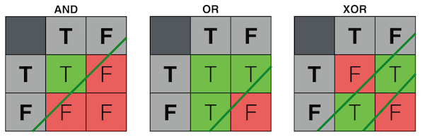
With AND and OR, a single cut (or "decision plane") separates the two output categories.
With XOR, we need two cuts. There is a mutual dependence between our inputs. We cannot simply look at each input dimension individually. If one is on, the other must be off.
For this reason, AND and OR are said to be linearly separable because their output space can be divided by a single line.
XOR, on the other hand, is not linearly seperable.
Interpretation
Complex ideas often contain interrelated components.
Therefore, to learn complex ideas, we need some way of accounting for these kinds of interrelations.
Yet these interrelations may not be obvious simply by looking at the data itself.
What we need, in essence, is a strategy for allowing the machine to invent new dimensions whose express purpose is to characterize the interdependency between the "actual" data dimensions.
We'll talk more about these "hidden dimensions" in the coming weeks.
Discussion
- What do these limitations tell us about the nature of learning?
- What conceptual alterations to the model might help to address these limitations?
Calculus Primer
Calculus is about approximating the analog world.
Zeno's Paradox of the Tortoise and Achilles
Integrals
Finding the area under the curve of a function

As \(\Delta{x} \rightarrow 0\), the area approximation will become more accurate and approach the true answer.
Finding an integral is the reverse of finding a derivative.
Notation
\(\textstyle \underbrace{\int}_{\text{(integral symbol)}} \underbrace{f(x)}_{\text{(function we want to integrate)}} \ \underbrace{dx}_{\text{(number of slices along x)}}\)
Notation Example
\(\displaystyle \int 2x \ dx = x^2 + C\)
where C is the constant of integration.
We need the constant of integration because, in this example, no matter what C equals, its derivative will equal 2x.
\(x^2 + 4\) becomes \(2x\)
\(x^2 + 6\) becomes \(2x\)
The constant is a placeholder for the information lost in converting from the derivative.
Derivatives
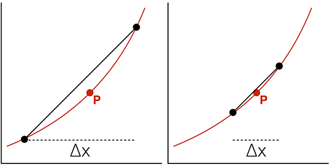
\(Slope = \frac{\Delta{y}}{\Delta{x}}\)
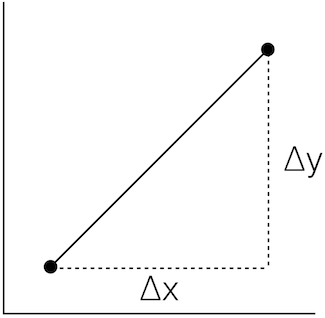
We can find an average slope between two points in order to approximate a curve:
\(Slope = \frac{\Delta{y}}{\Delta{x}} = \frac{3}{4} = 0.75\)
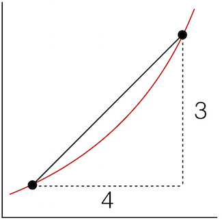
But this probably isn't a very good approximation of the curve.
To improve the approximation, we would like to use the smallest \(\Delta{x}\) possible.
Ideally, we would like to know the change in y at an individual x position: the instantaneous rate of change.
where \(\Delta{x} \rightarrow 0\).
\(\frac{\Delta{y}}{\Delta{x}} = \frac{f(x + \Delta{x}) - f(x)}{\Delta{x}}\)
where \(\Delta{x} \rightarrow 0\).
Example
Assume: \(f(x) = x^2\)
\( \require{cancel} \begin{align} \frac{\Delta{y}}{\Delta{x}} & = \frac{(x + \Delta{x})^2 - (x)^2}{\Delta{x}} \\ \\ & = \frac{\cancel{x^2} + 2x \Delta{x} + (\Delta{x})^2 - \cancel{x^2}}{\Delta{x}} \\ \\ & = \frac{2x \cancel{\Delta{x}} + (\Delta{x})^{\cancel{2}}}{\cancel{\Delta{x}}} \\ \\ & = 2x + \Delta{x} \\ \\ & \ {as} \ \Delta{x} \rightarrow 0, \\ & = 2x \end{align} \)
Derivative of \(x^2\) is \(2x\).
Notation
\(\frac{\mathrm{d}}{\mathrm{dx}} x^2 = 2x\)
For the function \(x^2\), the slope or "rate of change" at any point is 2x.
(Another) Notation
\( \begin{align} f(x) & = x^2 \\ f'(x) & = 2x \end{align} \)
The derivative of f equals the limit as \(\Delta{x}\) goes to zero of \(\frac{f(x + \Delta{x}) - f(x)}{\Delta{x}}\):
\( \begin{align} f'(x) & = \lim\limits_{\Delta{x} \to 0} \frac{f(x + \Delta{x}) - f(x)}{\Delta{x}} \\ \\ \frac{\mathrm{dy}}{\mathrm{dx}} & = \frac{f(x + dx) - f(x)}{dx} \\ \\ \end{align} \)
Symbolic Computation of Derivatives
Power Rule
\(\frac{d}{dx} \ x^n = n{x}^{n-1}\)
Sum Rule
The derivative of \(f + g = f' + g'\)
So, using the power rule, the derivative of \(x^2 + x^3 = 2x + 3x^2\)
Difference Rule
The derivative of \(f - g = f' - g'\)
Product Rule
The derivative of \(fg = fg' - f'g\)
Reciprocal Rule
The derivative of \(\frac{1}{f} = \frac{-f'}{f^2}\)
Chain Rule
The derivative of \(f(g(x)) = f'(g(x))g'(x)\)
Sin and Cos
\( \begin{align} \frac{d}{dx} sin(x) & = cos(x) \\ \\ \frac{d}{dx} cos(x) & = -sin(x) \\ \end{align} \)
Numerical Computation of Derivatives
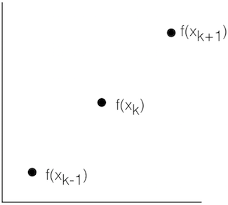
Forward Difference
\(f'(x_k) \approx \frac{f(x_{k+1})-f(x_k)}{x_{k+1}-x_k}\)
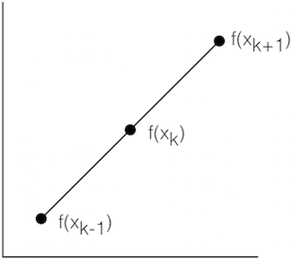
Central Difference
\(f'(x_k) \approx \frac{f(x_{k+1})-f(x_{k-1})}{x_{k+1}-x_{k-1}}\)
Numerical Differentiation in Python and Numpy
import numpy as np
import matplotlib.pyplot as plt

def func(x):
    return np.sin(x)

def dfunc(x):
    return np.cos(x)

xData = np.arange( -10.0, 10.0, 0.1 )
yData = func( xData )
yDeriv = dfunc( xData )
yDerivApprox = np.diff( yData ) / np.diff( xData )

plt.axis( [ -10.0, 10.0, -1.1, 1.1 ] )
plt.plot( xData, yData, 'r', xData, yDeriv, 'g', xData[0:len(xData)-1], yDerivApprox, 'b--' )
plt.show()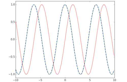
Partial Derivatives
Going into 3 dimensions...
Defining a 3D Surface
We can define z as a function of x and y:
\(z = f(x, y)\)
For example:
\( \begin{align} z & = x^2 + y \\ \\ z & = f(2, 1) \\ \\ & = 2^2 + 1 \\ \\ & = 5 \\ \\ \end{align} \)
How do we apply calculus to surfaces?
How would we find the slope for a given point on a surface in 3D?
This question isn't meaningful! We could find infinite tangents to the point.
So, when you take a derivative in 3D, you have to specify the direction that you're taking it in.
Example surface: \(z = x^2 + xy + y^2\)
We have to pick a direction, hold everything else constant and take a derivative with respect to just one variable.
This is called the Partial Derivative.
For: \(z = x^2 + xy + y^2\)
we will take the derivative of x and assume y is a constant.
Partial derivative of z with respect to x:
\( \textstyle \frac{\partial{z}}{\partial{x}} = \underbrace{2x}_{(x^2 \text{ becomes } 2x)} + \underbrace{y}_{(x \text{ drops power to become constant 1. } y \text{ is a constant so we keep it.})} \underbrace{\text{ }}_{(y \text{ is a constant. so is } y^2 \text{, so it becomes zero.} )} \)
Another notation:
\( \begin{align} f(x, y) & = x^2 + xy + y^2 \\ \\ f_x(x, y) & = 2x + y \\ \\ \end{align} \)
Now, partial derivative of z with respect to y:
\( \textstyle \frac{\partial{z}}{\partial{y}} = x + 2y \)
Homework
Assignment
- Implement a Perceptron in Python.
Readings
- Learning Internal Representations by Error Propagation by David Rumelhart, Geoffrey Hinton and Ronald Williams
- The Nature of Code by Daniel Shiffman, Chapter 10: "Neural Networks"
- Computational Neuroscience and Cognitive Modelling, Chapter 11: "An Introduction to Neural Networks"