Learning Machines: Week 2 — Linear Algebra & Classification

Linear Algebra Primer

Notation

Scalar: x (lowercase, regular)
Vector: \(\mathbf{u}\) (lowercase, bold)
Vector: \(\overrightarrow{u}\) (lowercase, w/ arrow)
Matrix: \(\mathbf{A}\) (uppercase, bold)

Summation: \(\sum\)
Product: \(\prod\)

Vector Definition

Formal Definition

n-tuple of values (usually real numbers) where n is the dimension of the vector and can be any positive integer \(\ge\) 1.

A vector can be thought of as...

a point in space
a directed line segment with a magnitude and direction

Formatting

Vectors can be written in column form or row form
Column form is conventional
Vector elements are referenced by subscript

Column Vector

\( \mathbf{x} = \begin{bmatrix} x_1 \\ \vdots \\ x_n \\ \end{bmatrix} \)

Row Vector

\( \mathbf{x} = \begin{bmatrix} x_1 \cdots x_n \end{bmatrix} \)

Transpose Row Vector to Column Vector

\( \begin{bmatrix} x_1 \cdots x_n \end{bmatrix}^\text{T} = \begin{bmatrix} x_1 \\ \vdots \\ x_n \\ \end{bmatrix} \)

Transpose Column Vector to Row Vector

\( \begin{bmatrix} x_1 \\ \vdots \\ x_n \\ \end{bmatrix}^\text{T} = \begin{bmatrix} x_1 \cdots x_n \end{bmatrix} \)

Vector Properties

Vectors are commutative: ( \(\overrightarrow{u}\) + \(\overrightarrow{v}\) ) is equal to ( \(\overrightarrow{v}\) + \(\overrightarrow{u}\) )
Vectors are associative: ( \(\overrightarrow{u}\) + ( \(\overrightarrow{v}\) + \(\overrightarrow{w}\) ) ) is equal to ( ( \(\overrightarrow{u}\) + \(\overrightarrow{v}\) ) + \(\overrightarrow{w}\) )

Working with Vectors and Matrices in Python and Numpy

Importing Numpy library

import numpy as np

Array Creation

>>> np.array( [ 0, 2, 4, 6, 8 ] )
array([0, 2, 4, 6, 8])

>>> np.zeros( 5 )
array([ 0.,  0.,  0.,  0.,  0.])

>>> np.ones( 5 )
array([ 1.,  1.,  1.,  1.,  1.])

>>> np.zeros( ( 5, 1 ) )
array([[ 0.],
       [ 0.],
       [ 0.],
       [ 0.],
       [ 0.]])

>>> np.zeros( ( 1, 5 ) )
array([[ 0.,  0.,  0.,  0.,  0.]])

>>> np.arange( 5 )
array([0, 1, 2, 3, 4])

>>> np.arange( 0, 1, 0.1 )
array([ 0. ,  0.1,  0.2,  0.3,  0.4,  0.5,  0.6,  0.7,  0.8,  0.9])

>>> np.linspace( 0, 1, 5 )
array([ 0.  ,  0.25,  0.5 ,  0.75,  1.  ])

>>> np.random.random( 5 )
array([ 0.22035712,  0.89856076,  0.46510509,  0.36395359,  0.3459122 ])

Vector Addition
Add corresponding elements. Result is a vector.

\[ \overrightarrow{z} = \overrightarrow{x} + \overrightarrow{y} = \begin{bmatrix} x_1 + y_1 \cdots x_n + y_n \end{bmatrix}^\text{T} \]

>>> x = np.array( [  1.0,  2.0,  3.0,  4.0,  5.0 ] )
>>> y = np.array( [ 10.0, 20.0, 30.0, 40.0, 50.0 ] )
>>> z = x + y
>>> z
array([ 11.,  22.,  33.,  44.,  55.])

Vector Subtraction
Subtract corresponding elements. Result is a vector.

\[ \overrightarrow{z} = \overrightarrow{x} - \overrightarrow{y} = \begin{bmatrix} x_1 - y_1 \cdots x_n - y_n \end{bmatrix}^\text{T} \]

>>> x = np.array( [  1.0,  2.0,  3.0,  4.0,  5.0 ] )
>>> y = np.array( [ 10.0, 20.0, 30.0, 40.0, 50.0 ] )
>>> z = x - y
>>> z
array([ -9., -18., -27., -36., -45.])

Vector Hadamard Product
Multiply corresponding elements. Result is a vector.

\[ \overrightarrow{z} = \overrightarrow{x} \circ \overrightarrow{y} = \begin{bmatrix} x_1 y_1 \cdots x_n y_n \end{bmatrix}^\text{T} \]

>>> x = np.array( [  1.0,  2.0,  3.0,  4.0,  5.0 ] )
>>> y = np.array( [ 10.0, 20.0, 30.0, 40.0, 50.0 ] )
>>> z = x * y
>>> z
array([  10.,   40.,   90.,  160.,  250.])

Vector Dot Product
Multiply corresponding elements, then add products. Result is a scalar.

\[ a = \overrightarrow{x} \cdot \overrightarrow{y} = \sum_{i=1}^n x_i y_i \]

>>> x = np.array( [  1.0,  2.0,  3.0,  4.0,  5.0 ] )
>>> y = np.array( [ 10.0, 20.0, 30.0, 40.0, 50.0 ] )
>>> a = np.dot( x, y )
>>> a
550.0

Vector-Scalar Addition
Add scalar to each element. Result is a vector.

\[ \overrightarrow{y} = \overrightarrow{x} + a = \begin{bmatrix} x_1 + a \cdots x_n + a \end{bmatrix}^\text{T} \]

>>> x = np.array( [  1.0,  2.0,  3.0,  4.0,  5.0 ] )
>>> a = 3.14
>>> y = x + a
>>> y
array([ 4.14,  5.14,  6.14,  7.14,  8.14])

Vector-Scalar Subtraction
Subtract scalar from each element. Result is a vector.

\[ \overrightarrow{y} = \overrightarrow{x} - a = \begin{bmatrix} x_1 - a \cdots x_n - a \end{bmatrix}^\text{T} \]

>>> x = np.array( [  1.0,  2.0,  3.0,  4.0,  5.0 ] )
>>> a = 3.14
>>> y = x - a
>>> y
array([-2.14, -1.14, -0.14,  0.86,  1.86])

Vector-Scalar Multiplication
Multiply each element by scalar. Result is a vector.

\[ \overrightarrow{y} = \overrightarrow{x} \ a = \begin{bmatrix} x_1 a \cdots x_n a \end{bmatrix}^\text{T} \]

>>> x = np.array( [  1.0,  2.0,  3.0,  4.0,  5.0 ] )
>>> a = 3.14
>>> y = x * a
>>> y
array([  3.14,   6.28,   9.42,  12.56,  15.7 ])

Vector-Scalar Division
Divide each element by scalar. Result is a vector.

\[ \overrightarrow{y} = \frac{\overrightarrow{x}}{a} = \begin{bmatrix} \frac{x_1}{a} \cdots \frac{x_n}{a} \end{bmatrix}^\text{T} \]

>>> x = np.array( [  1.0,  2.0,  3.0,  4.0,  5.0 ] )
>>> a = 3.14
>>> y = x / a
>>> y
array([ 0.31847134,  0.63694268,  0.95541401,  1.27388535,  1.59235669])

Vector Magnitude
Compute vector length. Result is a scalar.

\[ a = || \overrightarrow{x} || = \sqrt{ x_1^2 + \cdots + x_n^2 } = \sqrt{ \overrightarrow{x} \cdot \overrightarrow{x} } \]

>>> x = np.array( [  1.0,  2.0,  3.0,  4.0,  5.0 ] )
>>> a = np.linalg.norm( x )
>>> a
7.416198487095663

Vector Normalization
Compute unit vector. Result is a vector.

\[ \hat{x} = \frac{\overrightarrow{x}}{|| \overrightarrow{x} ||} \]

>>> x = np.array( [  1.0,  2.0,  3.0,  4.0,  5.0 ] )
>>> a = np.linalg.norm( x )
>>> x = x / a
>>> x
array([ 0.13483997,  0.26967994,  0.40451992,  0.53935989,  0.67419986])

Matrix Transposition
Swaps the row and column index for each element. For an m x n matrix, result is an n x m matrix.

\[ \mathbf{Y} = \mathbf{X}^\text{T} \]

>>> X = np.array( [ [ 1.0, 2.0, 3.0 ], [ 4.0, 5.0, 6.0 ] ] )
>>> Y = X.T
>>> Y
array([[ 1.,  4.],
       [ 2.,  5.],
       [ 3.,  6.]])

Matrix Addition
Add corresponding elements. Result is a matrix.

\[ \mathbf{Z} = \mathbf{X} + \mathbf{Y} = \begin{bmatrix} x_{11} + y_{11} & x_{12} + y_{12} & \cdots & x_{1n} + y_{1n} \\ x_{21} + y_{21} & x_{22} + y_{22} & \cdots & x_{2n} + y_{2n} \\ \vdots & \vdots & \ddots & \vdots \\ x_{m1} + y_{m1} & x_{m2} + y_{m2} & \cdots & x_{mn} + y_{mn} \\ \end{bmatrix} \]

>>> X = np.array( [ [  1.0,  2.0,  3.0 ], [  4.0,  5.0,  6.0 ] ] )
>>> Y = np.array( [ [ 10.0, 20.0, 30.0 ], [ 40.0, 50.0, 60.0 ] ] )
>>> Z = X + Y
>>> Z
array([[ 11.,  22.,  33.],
       [ 44.,  55.,  66.]])

Matrix Subtraction
Subtract corresponding elements. Result is a matrix.

\[ \mathbf{Z} = \mathbf{X} - \mathbf{Y} = \begin{bmatrix} x_{11} - y_{11} & x_{12} - y_{12} & \cdots & x_{1n} - y_{1n} \\ x_{21} - y_{21} & x_{22} - y_{22} & \cdots & x_{2n} - y_{2n} \\ \vdots & \vdots & \ddots & \vdots \\ x_{m1} - y_{m1} & x_{m2} - y_{m2} & \cdots & x_{mn} - y_{mn} \\ \end{bmatrix} \]

>>> X = np.array( [ [  1.0,  2.0,  3.0 ], [  4.0,  5.0,  6.0 ] ] )
>>> Y = np.array( [ [ 10.0, 20.0, 30.0 ], [ 40.0, 50.0, 60.0 ] ] )
>>> Z = X - Y
>>> Z
array([[ -9., -18., -27.],
       [-36., -45., -54.]])

Matrix Hadamard Product
Multiply corresponding elements. Result is a matrix.

\[ \mathbf{Z} = \mathbf{X} \circ \mathbf{Y} = \begin{bmatrix} x_{11} y_{11} & x_{12} y_{12} & \cdots & x_{1n} y_{1n} \\ x_{21} y_{21} & x_{22} y_{22} & \cdots & x_{2n} y_{2n} \\ \vdots & \vdots & \ddots & \vdots \\ x_{m1} y_{m1} & x_{m2} y_{m2} & \cdots & x_{mn} y_{mn} \\ \end{bmatrix} \]

>>> X = np.array( [ [  1.0,  2.0,  3.0 ], [  4.0,  5.0,  6.0 ] ] )
>>> Y = np.array( [ [ 10.0, 20.0, 30.0 ], [ 40.0, 50.0, 60.0 ] ] )
>>> Z = X * Y
>>> Z
array([[  10.,   40.,   90.],
       [ 160.,  250.,  360.]])

Matrix Multiplication
See Understanding Matrix Multiplication section.

\[ \begin{align} \mathbf{Z} & = \mathbf{X} \cdot \mathbf{Y} \\ \\ & = \begin{bmatrix} x_{11} & x_{12} & \cdots & x_{1n} \\ x_{21} & x_{22} & \cdots & x_{2n} \\ \vdots & \vdots & \ddots & \vdots \\ x_{m1} & x_{m2} & \cdots & x_{mn} \\ \end{bmatrix} \begin{bmatrix} y_{11} & y_{12} & \cdots & y_{1p} \\ y_{21} & y_{22} & \cdots & y_{2p} \\ \vdots & \vdots & \ddots & \vdots \\ y_{n1} & y_{n2} & \cdots & y_{np} \\ \end{bmatrix} \\ \\ & = \begin{bmatrix} x_{11} y_{11} + x_{12} y_{21} + \cdots + x_{1n} y_{n1} & x_{11} y_{12} + x_{12} y_{22} + \cdots + x_{1n} y_{n2} & \cdots & x_{11} y_{1p} + x_{12} y_{2p} + \cdots + x_{1n} y_{np} \\ x_{21} y_{11} + x_{22} y_{21} + \cdots + x_{2n} y_{n1} & x_{21} y_{12} + x_{22} y_{22} + \cdots + x_{2n} y_{n2} & \cdots & x_{21} y_{1p} + x_{22} y_{2p} + \cdots + x_{2n} y_{np} \\ \vdots & \vdots & \ddots & \vdots \\ x_{m1} y_{11} + x_{m2} y_{21} + \cdots + x_{mn} y_{n1} & x_{m1} y_{12} + x_{m2} y_{22} + \cdots + x_{mn} y_{n2} & \cdots & x_{m1} y_{1p} + x_{m2} y_{2p} + \cdots + x_{mn} y_{np} \\ \end{bmatrix} \\ \\ \end{align} \]

>>> X = np.array( [ [ 2, -4, 6 ], [ 5, 7, -3 ] ] )
>>> Y = np.array( [ [ 8, -5 ], [ 9, 3 ], [ -1, 4 ] ] )
>>> Z = np.dot( X, Y )
>>> Z
array([[-26,   2],
       [106, -16]])

Matrix-Scalar Addition
Add scalar to each element. Result is a matrix.

\[ \mathbf{Y} = \mathbf{X} + a = \begin{bmatrix} x_{11} + a & x_{12} + a & \cdots & x_{1n} + a \\ x_{21} + a & x_{22} + a & \cdots & x_{2n} + a \\ \vdots & \vdots & \ddots & \vdots \\ x_{m1} + a & x_{m2} + a & \cdots & x_{mn} + a \\ \end{bmatrix} \]

>>> X = np.array( [ [ 1.0, 2.0, 3.0 ], [ 4.0, 5.0, 6.0 ] ] )
>>> a = 3.14
>>> Y = X + a
>>> Y
array([[ 4.14,  5.14,  6.14],
       [ 7.14,  8.14,  9.14]])

Matrix-Scalar Subtraction
Subtract scalar from each element. Result is a matrix.

\[ \mathbf{Y} = \mathbf{X} - a = \begin{bmatrix} x_{11} - a & x_{12} - a & \cdots & x_{1n} - a \\ x_{21} - a & x_{22} - a & \cdots & x_{2n} - a \\ \vdots & \vdots & \ddots & \vdots \\ x_{m1} - a & x_{m2} - a & \cdots & x_{mn} - a \\ \end{bmatrix} \]

>>> X = np.array( [ [ 1.0, 2.0, 3.0 ], [ 4.0, 5.0, 6.0 ] ] )
>>> a = 3.14
>>> Y = X - a
>>> Y
array([[-2.14, -1.14, -0.14],
       [ 0.86,  1.86,  2.86]])

Matrix-Scalar Multiplication
Multiply each element by scalar. Result is a matrix.

\[ \mathbf{Y} = \mathbf{X} a = \begin{bmatrix} x_{11} a & x_{12} a & \cdots & x_{1n} a \\ x_{21} a & x_{22} a & \cdots & x_{2n} a \\ \vdots & \vdots & \ddots & \vdots \\ x_{m1} a & x_{m2} a & \cdots & x_{mn} a \\ \end{bmatrix} \]

>>> X = np.array( [ [ 1.0, 2.0, 3.0 ], [ 4.0, 5.0, 6.0 ] ] )
>>> a = 3.14
>>> Y = X * a
>>> Y
array([[  3.14,   6.28,   9.42],
       [ 12.56,  15.7 ,  18.84]])

Matrix-Scalar Division
Divide each element by scalar. Result is a matrix.

\[ \mathbf{Y} = \frac{\mathbf{X}}{a} = \begin{bmatrix} \frac{x_{11}}{a} & \frac{x_{12}}{a} & \cdots & \frac{x_{1n}}{a} \\ \frac{x_{21}}{a} & \frac{x_{22}}{a} & \cdots & \frac{x_{2n}}{a} \\ \vdots & \vdots & \ddots & \vdots \\ \frac{x_{m1}}{a} & \frac{x_{m2}}{a} & \cdots & \frac{x_{mn}}{a} \\ \end{bmatrix} \]

>>> X = np.array( [ [ 1.0, 2.0, 3.0 ], [ 4.0, 5.0, 6.0 ] ] )
>>> a = 3.14
>>> Y = X / a
>>> Y
array([[ 0.31847134,  0.63694268,  0.95541401],
       [ 1.27388535,  1.59235669,  1.91082803]])

Additional Documentation

Understanding Matrix Multiplication

The term matrix multiplication can be a bit confusing because its meaning is not consistent with matrix addition and matrix subtraction.

In matrix addition, we take two \(m\) x \(n\) matrices and add their corresponding elements, which results in another \(m\) x \(n\) matrix. Matrix subtraction works similarly.

So, it would seem to follow that matrix multiplication would have a similar meaning - that you multiply the corresponding elements. This operation, however, is not called matrix multiplication. It is instead called the Hadamard Product.

So what is matrix multiplication?

Matrix multiplication is a row-by-column operation in which the elements in the \(i^{th}\) row of the first matrix are multiplied by the corresponding elements of the \(j^{th}\) column of the second matrix and the results are added together.

For example, if we want to multiply these two matrices:

\( \begin{bmatrix} \color{blue}{2} & \color{blue}{-4} & \color{blue}{6} \\ 5 & 7 & -3 \\ \end{bmatrix} \begin{bmatrix} \color{green}{8} & -5 \\ \color{green}{9} & 3 \\ \color{green}{-1} & 4 \\ \end{bmatrix} \\ \\ \)

To compute the first element of the resulting matrix, we perform:

\( ( 2 * 8 ) + ( -4 * 9 ) + ( 6 * -1 ) = -26 \)

And insert this value into the resulting matrix:

\( \begin{bmatrix} -26 & ? \\ ? & ? \\ \end{bmatrix} \\ \\ \)

We follow this same form for each subsequent row-column pairing:

\( \begin{align} \begin{bmatrix} 2 & -4 & 6 \\ 5 & 7 & -3 \\ \end{bmatrix} \begin{bmatrix} 8 & -5 \\ 9 & 3 \\ -1 & 4 \\ \end{bmatrix} & = \begin{bmatrix} \mathbf{X}_{row1} \cdot \mathbf{Y}_{col1} & \mathbf{X}_{row1} \cdot \mathbf{Y}_{col2} \\ \mathbf{X}_{row2} \cdot \mathbf{Y}_{col1} & \mathbf{X}_{row2} \cdot \mathbf{Y}_{col2} \\ \end{bmatrix} \\ \\ & = \begin{bmatrix} (2)(8)+(-4)(9)+(6)(-1) & (2)(-5)+(-4)(3)+(6)(4) \\ (5)(8)+(7)(9)+(-3)(-1) & (5)(-5)+(7)(3)+(-3)(4) \\ \end{bmatrix} \\ \\ & = \begin{bmatrix} (16)+(-36)+(-6) & (-10)+(-12)+(24) \\ (40)+(63)+(3) & (-25)+(21)+(-12) \\ \end{bmatrix} \\ \\ & = \begin{bmatrix} -26 & 2 \\ 106 & -16 \\ \end{bmatrix} \\ \\ \end{align} \)

General Rules of Matrix Multiplication

\(\mathbf{X}_{mn} \cdot \mathbf{Y}_{np} = \mathbf{Z}_{mp}\)

The number of columns in \(\mathbf{X}\) must equal the number of rows in \(\mathbf{Y}\).
(Their inner dimensions must be the same)
The order of \(\mathbf{Z}\) is the number of rows in \(\mathbf{X}\) by the number of columns in \(\mathbf{Y}\).
(The dimensions of \(\mathbf{Z}\) are the outer dimensions)
Each element in row \(i\) of \(\mathbf{X}\) is paired with the corresponding element in column \(j\) of \(\mathbf{Y}\).
The element in row \(i\), column \(j\) of \(\mathbf{Z}\) is formed by multiplying these paired elements and summing the results.
For each element in \(\mathbf{Z}\), there will be \(n\) products that are summed.

Why is Matrix Multiplication Important?

At first glance, matrix multiplication seems to have a very specific definition, the value of which may not be obvious. Yet, matrix multiplication is one of the most commonly used operations in machine learning. Why? What does this seemingly obscure operation represent?

Matrix multiplication provides a natural mechanism for representing linear transformations.

For example, let's say we have a coordinate in two-dimensional space \(( x, y )\) that we wish to transform with the following formula:

\(Transform( x, y ) = (2x + 3y, 4x - 5y)\)

If \(( x, y ) = ( 7, 9 )\),
then \(Transform( 7, 9 ) = (2*7 + 3*9, 4*7 - 5*9) = (41, -17)\)

To represent \(Transform\) in matrix form, we create a matrix containing the coefficients of \(x\) and \(y\) like so:

\( Transform = \begin{bmatrix} 2 & 3 \\ 4 & -5 \\ \end{bmatrix} \\ \\ \)

We want to use this to produce our transformation: \(Transform( x, y ) = (2x + 3y, 4x - 5y)\)

Using matrix multiplication, we can write it like this:

\( \begin{bmatrix} 2 & 3 \\ 4 & -5 \\ \end{bmatrix} \begin{bmatrix} x \\ y \\ \end{bmatrix} = \begin{bmatrix} 2x + 3y \\ 4x - 5y \\ \end{bmatrix} \\ \\ \)

In this form, we could replace \(\begin{bmatrix} x \\ y \\ \end{bmatrix}\) with any specific \((x, y)\) pair in order to apply the transformation to that point. For example:

\( \begin{bmatrix} 2 & 3 \\ 4 & -5 \\ \end{bmatrix} \begin{bmatrix} 7 \\ 9 \\ \end{bmatrix} = \begin{bmatrix} 2*7 + 3*9 \\ 4*7 - 5*9 \\ \end{bmatrix} = \begin{bmatrix} 41 \\ -17 \\ \end{bmatrix} \\ \\ \)

Getting Started with Plotting in Python and Matplotlib

Importing Numpy library

import numpy as np

Importing Pyplot library

import matplotlib.pyplot as plt

Plot y-axis data

# Note: x-axis is automatically generated as [ 0, 1, 2, 3 ]

plt.plot( [ 1, 4, 9, 16 ] )
plt.show()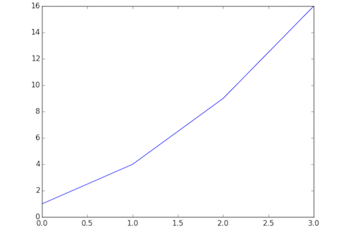

plot_yaxis

Plot x-axis and y-axis data

plt.plot( [ 1, 2, 3, 4 ], [ 1, 4, 9, 16 ] )
plt.show()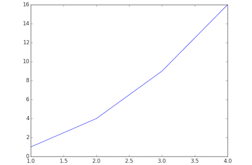

plot_xyaxis

Plot x-axis and y-axis data with per-axis extents

# Note: axis() formatted as [ xmin, xmax, ymin, ymax ]

plt.axis( [ 0, 6, 0, 50 ] )
plt.plot( [ 1, 2, 3, 4 ], [ 1, 4, 9, 16 ] )
plt.show()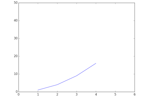

plot_xyaxis_ext

Customize axis labels

plt.xlabel('X-AXIS DATA')
plt.ylabel('Y-AXIS DATA')
plt.plot( [ 1, 2, 3, 4 ], [ 1, 4, 9, 16 ] )
plt.show()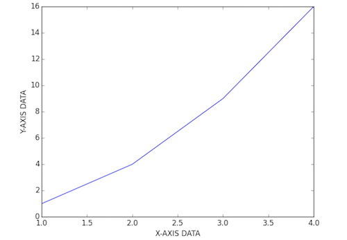

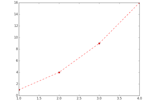
plot_custom_axis_labels

Customize plot stylization

plt.plot( [ 1, 2, 3, 4 ], [ 1, 4, 9, 16 ], 'ro--')
plt.show()

Additional documentation of stylization options can be found here: Pyplot Lines and Markers and Pyplot Line Properties

plot_custom_style

Plot functions

def sigmoid(x):
    return 1.0 / ( 1.0 + np.exp( -x ) )

def dsigmoid(x):
    y = sigmoid( x )
    return y * ( 1.0 - y )

def tanh(x):
    return np.sinh( x ) / np.cosh( x )

def dtanh(x):
    return 1.0 - np.square( tanh( x ) )

xData = np.arange( -10.0, 10.0, 0.1 )
ySigm = sigmoid( xData )
ySigd = dsigmoid( xData )
yTanh = tanh( xData )
yTand = dtanh( xData )

plt.axis( [ -10.0, 10.0, -1.1, 1.1 ] )
plt.plot( xData, ySigm, 'r', xData, ySigd, 'r--' )
plt.plot( xData, yTanh, 'g', xData, yTand, 'g--' )
plt.show()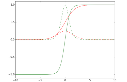

plot_custom_funcs

Working with multiple figures and axes

def f(t):
    return np.exp(-t) * np.cos(2*np.pi*t)

t1 = np.arange(0.0, 5.0, 0.1)
t2 = np.arange(0.0, 5.0, 0.02)

plt.figure(1)
plt.subplot(211)
plt.plot(t1, f(t1), 'bo', t2, f(t2), 'k')

plt.subplot(212)
plt.plot(t2, np.cos(2*np.pi*t2), 'r--')
plt.show()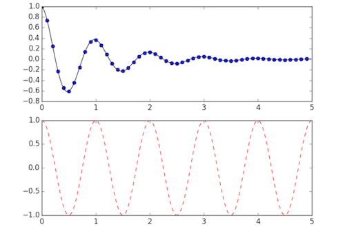

plot_subplots

Working with text

mu, sigma = 100, 15
x = mu + sigma * np.random.randn(10000)

# the histogram of the data
n, bins, patches = plt.hist(x, 50, normed=1, facecolor='g', alpha=0.75)

plt.xlabel('Smarts')
plt.ylabel('Probability')
plt.title('Histogram of IQ')
plt.text(60, .025, r'$\mu=100,\ \sigma=15$')
plt.axis([40, 160, 0, 0.03])
plt.grid(True)
plt.show()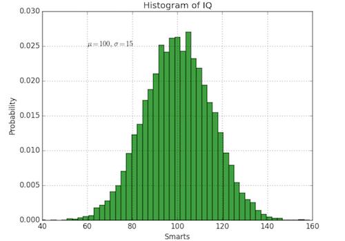

plot_text

ax = plt.subplot(111)

t = np.arange(0.0, 5.0, 0.01)
s = np.cos(2*np.pi*t)
line, = plt.plot(t, s, lw=2)

plt.annotate('local max', xy=(2, 1), xytext=(3, 1.5),
            arrowprops=dict(facecolor='black', shrink=0.05),
            )

plt.ylim(-2,2)
plt.show()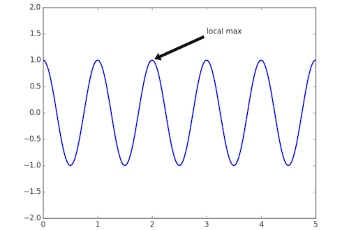

plot_annotation

Plotting in 3D

from mpl_toolkits.mplot3d import Axes3D
from matplotlib import cm
from matplotlib.ticker import LinearLocator, FormatStrFormatter

fig = plt.figure()
ax = fig.gca(projection='3d')
X = np.arange(-5, 5, 0.25)
Y = np.arange(-5, 5, 0.25)
X, Y = np.meshgrid(X, Y)
R = np.sqrt(X**2 + Y**2)
Z = np.sin(R)
surf = ax.plot_surface(X, Y, Z, rstride=1, cstride=1, cmap=cm.coolwarm,
                       linewidth=0, antialiased=False)
ax.set_zlim(-1.01, 1.01)

ax.zaxis.set_major_locator(LinearLocator(10))
ax.zaxis.set_major_formatter(FormatStrFormatter('%.02f'))

fig.colorbar(surf, shrink=0.5, aspect=5)

plt.show()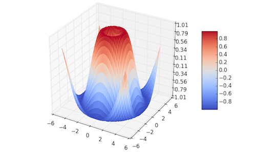

plot_3d

Additional Resources

Classification as Spatial Partitioning

CategoriesInPerception

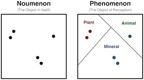
Classification can be a somewhat arbitrary process. It forces us to draw a line in the sand even though conceptual categories often have fuzzy boundaries. Presumably no one would say that one grain of sand makes a pile, but everyone would say one million grains of sand do. Somewhere between these, we must draw a line. In other words, categories are perceptual - their existence is contingent upon our looking for them. Let's see what this means for clustering algorithms.

A Brief Look at k-means Clustering

Concept

Assign data points to a set number of clusters:
- Find the nearest "cluster center" for each data point
- Adjust each cluster center position to be the centroid of its associated data points
- Repeat until no data point changes its assigned cluster from previous iteration

Algorithm

Let \( \mathbf{X} = \{ \mathbf{x_1}, \mathbf{x_2} \cdots \mathbf{x_n} \} \) be the set of data points
Let \( \mathbf{V} = \{ \mathbf{v_1}, \mathbf{v_2} \cdots \mathbf{v_c} \} \) be the set of cluster centers

Randomly select 'c' cluster centers
Compute the distance between each data point and each cluster center
Assign each data point to its nearest cluster
Recompute the new cluster centers using the formula:
\(\mathbf{v_i} = \frac{1}{c_i}\sum_{j=1}^{c_i} \mathbf{x_j}\)
where \(c_i\) is the number of data points in the \(i^{th}\) cluster
Recompute the distance between each data point and the new cluster centers
If no data point was reassigned then stop, otherwise repeat from Step 3

Limitations

Requires user to specify the number of clusters.
Therefore, we cannot really probe how many distinct categories exist.
Does not perform well on highly overlapping data.
Euclidean distance can skew weighting of underlying factors.
Algorithm is not invariant with respect to non-linear transformations.
With different representations of the data - polar coordinates vs Cartesian coordinates, e.g. - we get different results.

Additional Resources

Homework

Assignment

Install Python, Pip, NumPy and Matplotlib.
Implement K-Means Clustering in Python.
Spend some time experimenting with vectors and matrices in Python / NumPy:
- Try out the operations we've discussed.
- Plug-in different values and dimensions.
- Consider the results, tweak the values and repeat.
- The more you play with these operations, the more intuitive they will become.

Readings

The Perceptron: A Probabilistic Model for Information Storage and Organization in the Brain by Frank Rosenblatt