Taught by Patrick Hebron at ITP, Fall 2016
Homework Review
- Perceptron implementation
- Discussion of readings
Linear Algebra Primer (Part 2)
Notation:
Scalar: x (lowercase, regular)
Vector: \(\mathbf{u}\) (lowercase, bold)
Vector: \(\overrightarrow{u}\) (lowercase, w/ arrow)
Matrix: \(\mathbf{A}\) (uppercase, bold)
Summation: \(\sum\)
Product: \(\prod\)
Working with Matrices in Python and Numpy:
Importing Numpy library:
import numpy as npMatrix Transposition:
Swaps the row and column index for each element. For an m x n matrix, result is an n x m matrix.
\[ \mathbf{Y} = \mathbf{X}^\text{T} \]
>>> X = np.array( [ [ 1.0, 2.0, 3.0 ], [ 4.0, 5.0, 6.0 ] ] )
>>> Y = X.T
>>> Y
array([[ 1.,  4.],
       [ 2.,  5.],
       [ 3.,  6.]])
Matrix Addition:
Add corresponding elements. Result is a matrix.
\[ \mathbf{Z} = \mathbf{X} + \mathbf{Y} = \begin{bmatrix} x_{11} + y_{11} & x_{12} + y_{12} & \cdots & x_{1n} + y_{1n} \\ x_{21} + y_{21} & x_{22} + y_{22} & \cdots & x_{2n} + y_{2n} \\ \vdots & \vdots & \ddots & \vdots \\ x_{m1} + y_{m1} & x_{m2} + y_{m2} & \cdots & x_{mn} + y_{mn} \\ \end{bmatrix} \]
>>> X = np.array( [ [  1.0,  2.0,  3.0 ], [  4.0,  5.0,  6.0 ] ] )
>>> Y = np.array( [ [ 10.0, 20.0, 30.0 ], [ 40.0, 50.0, 60.0 ] ] )
>>> Z = X + Y
>>> Z
array([[ 11.,  22.,  33.],
       [ 44.,  55.,  66.]])
Matrix Subtraction:
Subtract corresponding elements. Result is a matrix.
\[ \mathbf{Z} = \mathbf{X} - \mathbf{Y} = \begin{bmatrix} x_{11} - y_{11} & x_{12} - y_{12} & \cdots & x_{1n} - y_{1n} \\ x_{21} - y_{21} & x_{22} - y_{22} & \cdots & x_{2n} - y_{2n} \\ \vdots & \vdots & \ddots & \vdots \\ x_{m1} - y_{m1} & x_{m2} - y_{m2} & \cdots & x_{mn} - y_{mn} \\ \end{bmatrix} \]
>>> X = np.array( [ [  1.0,  2.0,  3.0 ], [  4.0,  5.0,  6.0 ] ] )
>>> Y = np.array( [ [ 10.0, 20.0, 30.0 ], [ 40.0, 50.0, 60.0 ] ] )
>>> Z = X - Y
>>> Z
array([[ -9., -18., -27.],
       [-36., -45., -54.]])
Matrix Hadamard Product:
Multiply corresponding elements. Result is a matrix.
\[ \mathbf{Z} = \mathbf{X} \circ \mathbf{Y} = \begin{bmatrix} x_{11} y_{11} & x_{12} y_{12} & \cdots & x_{1n} y_{1n} \\ x_{21} y_{21} & x_{22} y_{22} & \cdots & x_{2n} y_{2n} \\ \vdots & \vdots & \ddots & \vdots \\ x_{m1} y_{m1} & x_{m2} y_{m2} & \cdots & x_{mn} y_{mn} \\ \end{bmatrix} \]
>>> X = np.array( [ [  1.0,  2.0,  3.0 ], [  4.0,  5.0,  6.0 ] ] )
>>> Y = np.array( [ [ 10.0, 20.0, 30.0 ], [ 40.0, 50.0, 60.0 ] ] )
>>> Z = X * Y
>>> Z
array([[  10.,   40.,   90.],
       [ 160.,  250.,  360.]])
Matrix Multiplication:
See Understanding Matrix Multiplication section.
\[ \begin{align} \mathbf{Z} & = \mathbf{X} \cdot \mathbf{Y} \\ \\ & = \begin{bmatrix} x_{11} & x_{12} & \cdots & x_{1n} \\ x_{21} & x_{22} & \cdots & x_{2n} \\ \vdots & \vdots & \ddots & \vdots \\ x_{m1} & x_{m2} & \cdots & x_{mn} \\ \end{bmatrix} \begin{bmatrix} y_{11} & y_{12} & \cdots & y_{1p} \\ y_{21} & y_{22} & \cdots & y_{2p} \\ \vdots & \vdots & \ddots & \vdots \\ y_{n1} & y_{n2} & \cdots & y_{np} \\ \end{bmatrix} \\ \\ & = \begin{bmatrix} x_{11} y_{11} + x_{12} y_{21} + \cdots + x_{1n} y_{n1} & x_{11} y_{12} + x_{12} y_{22} + \cdots + x_{1n} y_{n2} & \cdots & x_{11} y_{1p} + x_{12} y_{2p} + \cdots + x_{1n} y_{np} \\ x_{21} y_{11} + x_{22} y_{21} + \cdots + x_{2n} y_{n1} & x_{21} y_{12} + x_{22} y_{22} + \cdots + x_{2n} y_{n2} & \cdots & x_{21} y_{1p} + x_{22} y_{2p} + \cdots + x_{2n} y_{np} \\ \vdots & \vdots & \ddots & \vdots \\ x_{m1} y_{11} + x_{m2} y_{21} + \cdots + x_{mn} y_{n1} & x_{m1} y_{12} + x_{m2} y_{22} + \cdots + x_{mn} y_{n2} & \cdots & x_{m1} y_{1p} + x_{m2} y_{2p} + \cdots + x_{mn} y_{np} \\ \end{bmatrix} \\ \\ \end{align} \]
>>> X = np.array( [ [ 2, -4, 6 ], [ 5, 7, -3 ] ] )
>>> Y = np.array( [ [ 8, -5 ], [ 9, 3 ], [ -1, 4 ] ] )
>>> Z = np.dot( X, Y )
>>> Z
array([[-26,   2],
       [106, -16]])
Matrix-Scalar Addition:
Add scalar to each element. Result is a matrix.
\[ \mathbf{Y} = \mathbf{X} + a = \begin{bmatrix} x_{11} + a & x_{12} + a & \cdots & x_{1n} + a \\ x_{21} + a & x_{22} + a & \cdots & x_{2n} + a \\ \vdots & \vdots & \ddots & \vdots \\ x_{m1} + a & x_{m2} + a & \cdots & x_{mn} + a \\ \end{bmatrix} \]
>>> X = np.array( [ [ 1.0, 2.0, 3.0 ], [ 4.0, 5.0, 6.0 ] ] )
>>> a = 3.14
>>> Y = X + a
>>> Y
array([[ 4.14,  5.14,  6.14],
       [ 7.14,  8.14,  9.14]])
Matrix-Scalar Subtraction:
Subtract scalar from each element. Result is a matrix.
\[ \mathbf{Y} = \mathbf{X} - a = \begin{bmatrix} x_{11} - a & x_{12} - a & \cdots & x_{1n} - a \\ x_{21} - a & x_{22} - a & \cdots & x_{2n} - a \\ \vdots & \vdots & \ddots & \vdots \\ x_{m1} - a & x_{m2} - a & \cdots & x_{mn} - a \\ \end{bmatrix} \]
>>> X = np.array( [ [ 1.0, 2.0, 3.0 ], [ 4.0, 5.0, 6.0 ] ] )
>>> a = 3.14
>>> Y = X - a
>>> Y
array([[-2.14, -1.14, -0.14],
       [ 0.86,  1.86,  2.86]])
Matrix-Scalar Multiplication:
Multiply each element by scalar. Result is a matrix.
\[ \mathbf{Y} = \mathbf{X} a = \begin{bmatrix} x_{11} a & x_{12} a & \cdots & x_{1n} a \\ x_{21} a & x_{22} a & \cdots & x_{2n} a \\ \vdots & \vdots & \ddots & \vdots \\ x_{m1} a & x_{m2} a & \cdots & x_{mn} a \\ \end{bmatrix} \]
>>> X = np.array( [ [ 1.0, 2.0, 3.0 ], [ 4.0, 5.0, 6.0 ] ] )
>>> a = 3.14
>>> Y = X * a
>>> Y
array([[  3.14,   6.28,   9.42],
       [ 12.56,  15.7 ,  18.84]])
Matrix-Scalar Division:
Divide each element by scalar. Result is a matrix.
\[ \mathbf{Y} = \frac{\mathbf{X}}{a} = \begin{bmatrix} \frac{x_{11}}{a} & \frac{x_{12}}{a} & \cdots & \frac{x_{1n}}{a} \\ \frac{x_{21}}{a} & \frac{x_{22}}{a} & \cdots & \frac{x_{2n}}{a} \\ \vdots & \vdots & \ddots & \vdots \\ \frac{x_{m1}}{a} & \frac{x_{m2}}{a} & \cdots & \frac{x_{mn}}{a} \\ \end{bmatrix} \]
>>> X = np.array( [ [ 1.0, 2.0, 3.0 ], [ 4.0, 5.0, 6.0 ] ] )
>>> a = 3.14
>>> Y = X / a
>>> Y
array([[ 0.31847134,  0.63694268,  0.95541401],
       [ 1.27388535,  1.59235669,  1.91082803]])
Additional Documentation:
Understanding Matrix Multiplication:
The term matrix multiplication can be a bit confusing because its meaning is not consistent with matrix addition and matrix subtraction.
In matrix addition, we take two \(m\) x \(n\) matrices and add their corresponding elements, which results in another \(m\) x \(n\) matrix.
Matrix subtraction works similarly to matrix addition, except you subtract the corresponding elements.
So, it would seem to follow that matrix multiplication would have a similar meaning - that you multiply the corresponding elements. This operation, however, is not called matrix multiplication. It is instead called the Hadamard Product.
So what is matrix multiplication?
Matrix multiplication is a row-by-column operation in which the elements in the \(i^{th}\) row of the first matrix are multiplied by the corresponding elements of the \(j^{th}\) column of the second matrix and the results are added together.
For example, if we want to multiply these two matrices:
\( \begin{bmatrix} \color{blue}{2} & \color{blue}{-4} & \color{blue}{6} \\ 5 & 7 & -3 \\ \end{bmatrix} \begin{bmatrix} \color{green}{8} & -5 \\ \color{green}{9} & 3 \\ \color{green}{-1} & 4 \\ \end{bmatrix} \\ \\ \)
To compute the first element of the resulting matrix, we perform:
\( ( 2 * 8 ) + ( -4 * 9 ) + ( 6 * -1 ) = -26 \)
And insert this value into the resulting matrix:
\( \begin{bmatrix} -26 & ? \\ ? & ? \\ \end{bmatrix} \\ \\ \)
We follow this same form for each subsequent row-column pairing:
\( \begin{align} \begin{bmatrix} 2 & -4 & 6 \\ 5 & 7 & -3 \\ \end{bmatrix} \begin{bmatrix} 8 & -5 \\ 9 & 3 \\ -1 & 4 \\ \end{bmatrix} & = \begin{bmatrix} \mathbf{X}_{row1} \cdot \mathbf{Y}_{col1} & \mathbf{X}_{row1} \cdot \mathbf{Y}_{col2} \\ \mathbf{X}_{row2} \cdot \mathbf{Y}_{col1} & \mathbf{X}_{row2} \cdot \mathbf{Y}_{col2} \\ \end{bmatrix} \\ \\ & = \begin{bmatrix} (2)(8)+(-4)(9)+(6)(-1) & (2)(-5)+(-4)(3)+(6)(4) \\ (5)(8)+(7)(9)+(-3)(-1) & (5)(-5)+(7)(3)+(-3)(4) \\ \end{bmatrix} \\ \\ & = \begin{bmatrix} (16)+(-36)+(-6) & (-10)+(-12)+(24) \\ (40)+(63)+(3) & (-25)+(21)+(-12) \\ \end{bmatrix} \\ \\ & = \begin{bmatrix} -26 & 2 \\ 106 & -16 \\ \end{bmatrix} \\ \\ \end{align} \)
General Rules of Matrix Multiplication:
\(\mathbf{X}_{mn} \cdot \mathbf{Y}_{np} = \mathbf{Z}_{mp}\)
- The number of columns in \(\mathbf{X}\) must equal the number of rows in \(\mathbf{Y}\).
(Their inner dimensions must be the same) - The order of \(\mathbf{Z}\) is the number of rows in \(\mathbf{X}\) by the number of columns in \(\mathbf{Y}\).
(The dimensions of \(\mathbf{Z}\) are the outer dimensions) - Each element in row \(i\) of \(\mathbf{X}\) is paired with the corresponding element in column \(j\) of \(\mathbf{Y}\).
- The element in row \(i\), column \(j\) of \(\mathbf{Z}\) is formed by multiplying these paired elements and summing the results.
- For each element in \(\mathbf{Z}\), there will be \(n\) products that are summed.
Why is Matrix Multiplication Important?:
At first glance, matrix multiplication seems to have a very specific definition, the value of which may not be obvious. Yet, matrix multiplication is one of the most commonly used operations in machine learning. Why? What does this seemingly obscure operation represent?
Matrix multiplication provides a natural mechanism for representing linear transformations.
For example, let's say we have a coordinate in two-dimensional space \(( x, y )\) that we wish to transform with the following formula:
\(Transform( x, y ) = (2x + 3y, 4x - 5y)\)
If \(( x, y ) = ( 7, 9 )\),
then \(Transform( 7, 9 ) = (2*7 + 3*9, 4*7 - 5*9) = (41, -17)\)
To represent \(Transform\) in matrix form, we create a matrix containing the coefficients of \(x\) and \(y\) like so:
\( Transform = \begin{bmatrix} 2 & 3 \\ 4 & -5 \\ \end{bmatrix} \\ \\ \)
We want to use this to produce our transformation: \(Transform( x, y ) = (2x + 3y, 4x - 5y)\)
Using matrix multiplication, we can write it like this:
\( \begin{bmatrix} 2 & 3 \\ 4 & -5 \\ \end{bmatrix} \begin{bmatrix} x \\ y \\ \end{bmatrix} = \begin{bmatrix} 2x + 3y \\ 4x - 5y \\ \end{bmatrix} \\ \\ \)
In this form, we could replace \(\begin{bmatrix} x \\ y \\ \end{bmatrix}\) with any specific \((x, y)\) pair in order to apply the transformation to that point. For example:
\( \begin{bmatrix} 2 & 3 \\ 4 & -5 \\ \end{bmatrix} \begin{bmatrix} 7 \\ 9 \\ \end{bmatrix} = \begin{bmatrix} 2*7 + 3*9 \\ 4*7 - 5*9 \\ \end{bmatrix} = \begin{bmatrix} 41 \\ -17 \\ \end{bmatrix} \\ \\ \)
Calculus Primer
Calculus is about approximating the analog world.
Zeno's Paradox of the Tortoise and Achilles
Integrals:
Finding the area under the curve of a function:
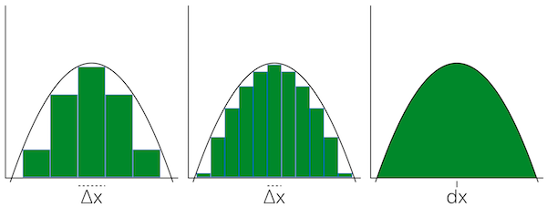
As \(\Delta{x} \rightarrow 0\), the area approximation will become more accurate and approach the true answer.
Finding an integral is the reverse of finding a derivative.
Notation:
\(\textstyle \underbrace{\int}_{\text{(integral symbol)}} \underbrace{f(x)}_{\text{(function we want to integrate)}} \ \underbrace{dx}_{\text{(number of slices along x)}}\)
Notation Example:
\(\displaystyle \int 2x \ dx = x^2 + C\)
where C is the constant of integration.
We need the constant of integration because, in this example, no matter what C equals, its derivative will equal 2x.
\(x^2 + 4\) becomes \(2x\)
\(x^2 + 6\) becomes \(2x\)
The constant is a placeholder for the information lost in converting from the derivative.
Derivatives:
\(Slope = \frac{\Delta{y}}{\Delta{x}}\)
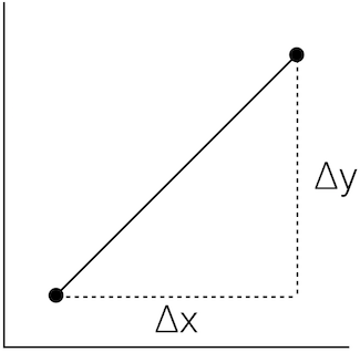
We can find an average slope between two points in order to approximate a curve:
\(Slope = \frac{\Delta{y}}{\Delta{x}} = \frac{3}{4} = 0.75\)

But this probably isn't a very good approximation of the curve.
To improve the approximation, we would like to use the smallest \(\Delta{x}\) possible.
Ideally, we would like to know the change in y at an individual x position: the instantaneous rate of change.
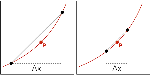
where \(\Delta{x} \rightarrow 0\).
\(\frac{\Delta{y}}{\Delta{x}} = \frac{f(x + \Delta{x}) - f(x)}{\Delta{x}}\)
where \(\Delta{x} \rightarrow 0\).
Example:
Assume: \(f(x) = x^2\)
\( \require{cancel} \begin{align} \frac{\Delta{y}}{\Delta{x}} & = \frac{(x + \Delta{x})^2 - (x)^2}{\Delta{x}} \\ \\ & = \frac{\cancel{x^2} + 2x \Delta{x} + (\Delta{x})^2 - \cancel{x^2}}{\Delta{x}} \\ \\ & = \frac{2x \cancel{\Delta{x}} + (\Delta{x})^{\cancel{2}}}{\cancel{\Delta{x}}} \\ \\ & = 2x + \Delta{x} \\ \\ & \ {as} \ \Delta{x} \rightarrow 0, \\ & = 2x \end{align} \)
Derivative of \(x^2\) is \(2x\).
Notation:
\(\frac{\mathrm{d}}{\mathrm{dx}} x^2 = 2x\)
For the function \(x^2\), the slope or "rate of change" at any point is 2x.
(Another) Notation:
\( \begin{align} f(x) & = x^2 \\ f'(x) & = 2x \end{align} \)
The derivative of f equals the limit as \(\Delta{x}\) goes to zero of \(\frac{f(x + \Delta{x}) - f(x)}{\Delta{x}}\):
\( \begin{align} f'(x) & = \lim\limits_{\Delta{x} \to 0} \frac{f(x + \Delta{x}) - f(x)}{\Delta{x}} \\ \\ \frac{\mathrm{dy}}{\mathrm{dx}} & = \frac{f(x + dx) - f(x)}{dx} \\ \\ \end{align} \)
Symbolic Computation of Derivatives:
Power Rule:
\(\frac{d}{dx} \ x^n = n{x}^{n-1}\)
Sum Rule:
The derivative of \(f + g = f' + g'\)
So, using the power rule, the derivative of \(x^2 + x^3 = 2x + 3x^2\)
Difference Rule:
The derivative of \(f - g = f' - g'\)
Product Rule:
The derivative of \(fg = fg' - f'g\)
Reciprocal Rule:
The derivative of \(\frac{1}{f} = \frac{-f'}{f^2}\)
Chain Rule:
The derivative of \(f(g(x)) = f'(g(x))g'(x)\)
Sin and Cos:
\( \begin{align} \frac{d}{dx} sin(x) & = cos(x) \\ \\ \frac{d}{dx} cos(x) & = -sin(x) \\ \end{align} \)
Numerical Computation of Derivatives:
Forward Difference:
\(f'(x_k) \approx \frac{f(x_{k+1})-f(x_k)}{x_{k+1}-x_k}\)
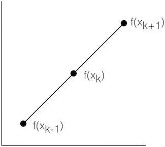
Central Difference:
\(f'(x_k) \approx \frac{f(x_{k+1})-f(x_{k-1})}{x_{k+1}-x_{k-1}}\)

Numerical Differentiation in Python and Numpy:
import numpy as np
import matplotlib.pyplot as plt

def func(x):
    return np.sin(x)

def dfunc(x):
    return np.cos(x)

xData = np.arange( -10.0, 10.0, 0.1 )
yData = func( xData )
yDeriv = dfunc( xData )
yDerivApprox = np.diff( yData ) / np.diff( xData )

plt.axis( [ -10.0, 10.0, -1.1, 1.1 ] )
plt.plot( xData, yData, 'r', xData, yDeriv, 'g', xData[0:len(xData)-1], yDerivApprox, 'b--' )
plt.show()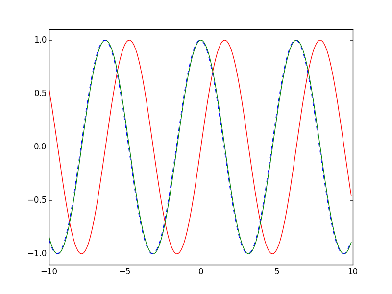
Partial Derivatives:
Going into 3 dimensions...
Defining a 3D Surface:
We can define z as a function of x and y:
\(z = f(x, y)\)
For example:
\( \begin{align} z & = x^2 + y \\ \\ z & = f(2, 1) \\ \\ & = 2^2 + 1 \\ \\ & = 5 \\ \\ \end{align} \)
How do we apply calculus to surfaces?
How would we find the slope for a given point on a surface in 3D?
This question isn't meaningful! We could find infinite tangents to the point.
So, when you take a derivative in 3D, you have to specify the direction that you're taking it in.
Example surface: \(z = x^2 + xy + y^2\)
We have to pick a direction, hold everything else constant and take a derivative with respect to just one variable.
This is called the Partial Derivative.
For: \(z = x^2 + xy + y^2\)
we will take the derivative of x and assume y is a constant.
Partial derivative of z with respect to x:
\( \textstyle \frac{\partial{z}}{\partial{x}} = \underbrace{2x}_{(x^2 \text{ becomes } 2x)} + \underbrace{y}_{(x \text{ drops power to become constant 1. } y \text{ is a constant so we keep it.})} \underbrace{\text{ }}_{(y \text{ is a constant. so is } y^2 \text{, so it becomes zero.} )} \)
Another notation:
\( \begin{align} f(x, y) & = x^2 + xy + y^2 \\ \\ f_x(x, y) & = 2x + y \\ \\ \end{align} \)
Now, partial derivative of z with respect to x:
\( \textstyle \frac{\partial{z}}{\partial{y}} = x + 2y \)
The Multilayer Perceptron (MLP)
Based on CSC321: Neural Networks, by Geoffrey Hinton.
Relation to Perceptrons:
Multilayer Perceptrons do not use the Perceptron learning algorithm.
As Geoff Hinton says, they never should have been called Multilayer Perceptrons because...
The Perceptron learning algorithm cannot be generalized to hidden layers.
Perceptron convergence works by ensuring that every time the weights change, they get closer to every "generously feasible" set of weights.
This type of guarantee cannot be extended to more complex networks in which the average of two good solutions may be a bad solution.
So, "multi-layer" networks do not use the Perceptron learning algorithm.
Demonstrating Progress:
Instead of showing that the weights are getting closer to a good set of weights,
show that the actual output values are getting closer to the target values.
This can be true even for non-convex problems where lots of different sets of weights could work well and averaging two good sets of weights may give a bad set of weights. It is not true of Perceptron learning.
Moving Beyond the Perceptron's Limitations:
Neural networks without any hidden units are very limited in what they can model.
Adding a layer of hand-picked features to Perceptrons makes them much more powerful.
But it is difficult to design good features, especially for a complex problem!
We want to find good features without requiring any human insights into the task. We also want to avoid repeated trial-and-error.
We need to automate the process of designing features for a specific task and seeing how well they work.
A First Attempt Using an Evolutionary Mindset:
Looking to the natural world for inspiration is often a good starting point.
Evolution provides an obvious point of entry to the problem of iteratively optimizing a set of weights in order to address a specific task.
As a basic sketch, we might consider a procedure like this:
- Randomly change one weight and see if it improves performance.
- If so, save the change and move on to the next weight.
Unfortunately, this approach is extremely inefficient.
To check whether a single weight change improves the system's performance, we need to compute at the predicted output for a large number of training examples.
Towards the end of the training process, large weight changes will usually make things worse because the weights need to have the right relative values to one another. One way to understand this problem is to imagine trying to solve a Rubik's Cube by getting a single face to be all one color, then moving to the next face. You end up undoing your earlier work!
Evolution is clearly a powerful mechanism in nature. But it also requires an immense amount of time. Ideally, we can find a more efficient approach!
We could try randomly changing all of the weights at the same time.
But this isn't any better because we would need to perform many trials on each training example in order to distinguish the impact on one weight from the noise created by changing all of the other weights. (Again, think of the Rubik's cube)
A better approach would be to make random changes to the hidden units' activities.
If we know how we want to change the hidden unit's activities for a specific training example, we can figure out how to change the weights accordingly.
Backpropagation Conceptual Overview:
We don't know exactly what we want the hidden units to do. But we can compute the rate of change in the prediction error as we change a hidden activity.
Rather than using the desired activities to train the hidden units, we will instead use error derivatives with respect to the hidden activities.
Each hidden activity will impact numerous output units and can therefore have many different effects upon the overall error. These effects must be combined.
We can efficiently compute error derivatives for all hidden units simultaneously.
Backpropagation Overview for a Single Training Example:
- Convert the difference between each output and its target value into an error derivative.
- Compute error derivatives in each hidden layer from error derivatives in previous layer.
- Use error derivatives with respect to activities to get error derivatives with respect to the incoming weights.
Let's now look at how to extend this to a full training procedure...
The Delta Rule:
\( \begin{align} \Delta{w} & = w - w_{old} \\ \\ & = - LearningConstant \frac{\partial{E}}{\partial{w}} \\ \\ & = (LearningConstant)(y_{target}-y)(x) \\ \\ \end{align} \)
or...
\( w = w_{old} + (LearningConstant)(y_{target}-y)(x) \)
The Delta Rule is similar to the Perceptron Learning Rule, but differs in the following ways:
- The error \((y_{target}-y)\) in the Delta Rule can have any value, not just \(0\), \(1\) or \(-1\).
- The Delta Rule can be derived for any differentiable activation function \(f\). The Perceptron Learning Rule only works for a threshold output function.
Multilayer Perceptron Architecture:
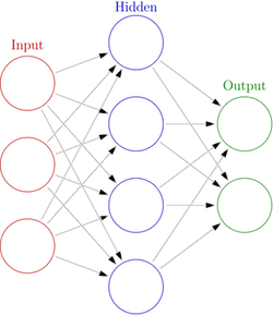
Each node in the hidden layer is a function of the nodes in the previous layer.
The output node is a function of the nodes in the hidden layer.
Multilayer Perceptron Training Procedure:
- Choose a number of training epochs.
- Choose a learning rate.
- Choose layer count and layer sizes. (Here, we will use only one hidden layer)
- Initialize random weights and biases for connections between the input and hidden layer.
- Initialize random weights and biases for connections between the hidden and output layer.
- For each training epoch:
- Choose a random input/output training example pair.
- Feed Forward:
- For input-to-hidden connections:
- Compute activations:
\(activations = weights \cdot input + bias\) - Compute outputs:
\(outputs = ActivationFn( activations )\)
- Compute activations:
- Do the same for hidden-to-output connections.
- For input-to-hidden connections:
- Back Propagation:
- For output-to-hidden connections:
- Compute deltas:
\(deltas = ActivationDerivativeFn( activations ) \circ ({Outputs}_{guessed} - {Outputs}_{actual})\)
- Compute deltas:
- For hidden-to-input connections:
- Compute deltas:
\(deltas = ActivationDerivativeFn( activations ) \circ ( {weights}^T \cdot OutputToHiddenDeltas)\)
- Compute deltas:
- For output-to-hidden connections:
- Updates:
- For input-to-hidden connections:
- Apply deltas:
\(weights = weights - LearningConstant ( deltas \cdot inputs )\)
\(bias = bias - LearningConstant ( deltas )\)
- Apply deltas:
- Do the same for hidden-to-output connections.
- For input-to-hidden connections:
Homework
Assignment:
- This week, I will provide an "unrolled" Multilayer Perceptron implementation in Python. This code implements a three-layer MLP (input, output and one hidden layer) in an easy-to-read format, but does not attempt to provide a generalized architecture for adding additional hidden layers, etc. Using this code as a starting point, please implement a more generalized solution. Your code should allow the user to specify the size of each layer and the number of hidden layers as well as provide a clear API for training and testing the model on user-provided datasets.
- Code: mlp_unrolled.py
Readings:
- Computational Neuroscience and Cognitive Modelling, Chapter 2: "What Is a Differential Equation?"
- Computational Neuroscience and Cognitive Modelling, Chapter 3: "Numerical Application of a Differential Equation"
- Primary Source: Reducing the Dimensionality of Data with Neural Networks by Geoffrey Hinton and R. R. Salakhutdinov