Week 3

Homework Review

• Recommendation engine
• Discussion of readings

Learning to Draw a Line in the Sand

Classification as Spatial Partitioning:

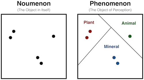
Classification can be a somewhat arbitrary process. It forces us to draw a line in the sand even though conceptual categories often have fuzzy boundaries. Presumably no one would say that one grain of sand makes a pile, but everyone would say one million grains of sand do. Somewhere between these, we must draw a line. In other words, categories are perceptual - their existence is contingent upon our looking for them. Let's see what this means for clustering algorithms.

A Brief Look at k-means Clustering:

Concept:

• Assign data points to a set number of clusters:
  • Find the nearest "cluster center" for each data point
  • Adjust each cluster center position to be the centroid of its associated data points
  • Repeat until no data point changes its assigned cluster from previous iteration

Algorithm:

• Let \( \mathbf{X} = \{ \mathbf{x_1}, \mathbf{x_2} \cdots \mathbf{x_n} \} \) be the set of data points

• Let \( \mathbf{V} = \{ \mathbf{v_1}, \mathbf{v_2} \cdots \mathbf{v_c} \} \) be the set of cluster centers

1. Randomly select 'c' cluster centers
2. Compute the distance between each data point and each cluster center
3. Assign each data point to its nearest cluster
4. Recompute the new cluster centers using the formula:
   \(\mathbf{v_i} = \frac{1}{c_i}\sum_{j=1}^{c_i} \mathbf{x_j}\)
   where \(c_i\) is the number of data points in the \(i^{th}\) cluster
5. Recompute the distance between each data point and the new cluster centers
6. If no data point was reassigned then stop, otherwise repeat from Step 3

Limitations:

• Requires user to specify the number of clusters.
  Therefore, we cannot really probe how many distinct categories exist.
• Does not perform well on highly overlapping data.
• Euclidean distance can skew weighting of underlying factors.
• Algorithm is not invariant with respect to non-linear transformations.
  With different representations of the data - polar coordinates vs Cartesian coordinates, e.g. - we get different results.

Additional Resources:

• K-Means Clustering Visualization
  
• K-Means Clustering Overview

Perceptrons

History:

• Perceptron algorithm invented by Frank Rosenblatt in 1957.
• Rosenblatt developed the algorithm for the US Office of Naval Research for image recognition purposes.
• Rosenblatt made bold claims about the future of Artificial Intelligence and the ability to teach machines to walk, talk, see, etc.
  This led to controversy.
• In 1969, Marvin Minsky and Seymour Papert published the book, Perceptrons, which conclusively showed that it was impossible for perceptrons to learn an exclusive-or (XOR) function.
• Minsky and Papert were aware that using multiple layers in the network would allow the representation of an XOR function. But the common misunderstanding of an artificial neural network's limitations led to a stark decline in interest and funding - an AI Winter.
• In the 1980s, interest grew again with work on Multilayer Perceptrons and the Backpropagation algorithm, developed by David Rumelhart, Geoff Hinton, et al.

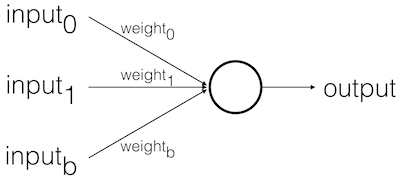
Basic Model:

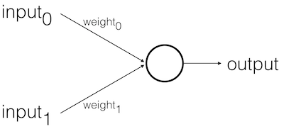
Feed Forward Stages:

1. Receive inputs
2. Weigh inputs
3. Sum inputs
4. Generate output

Example:

1. \(input_0\) = 12
   \(input_1\) = 4
   
   
2. (weights are initially random)
   \(weight_0\) = 0.5
   \(weight_1\) = -1.0
   
   \(input_0 * weight_0\) = 12 * 0.5 = 6
   \(input_1 * weight_1\) = 4 * -1.0 = -4
   
   
3. \(sum\) = 6 + -4 = 2
   
   
4. \(output\) = Sign( \(sum\) ) = Sign( 2 ) = +1

The Perceptron Algorithm:

1. For every input, multiply that input by its weight.
2. Sum all of the weighted inputs.
3. Compute the output based on that sum passed through an activation function
   Here, the activation function will be the sign of the sum.

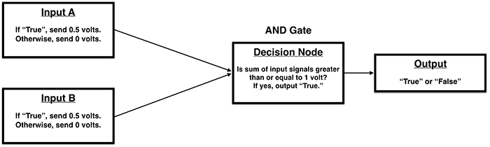
Electrical Analogy:

An electronic logic gate is a lot like a pre-trained Perceptron.

Consider Alan Turing's comment in Intelligent Machinery:
"Many unorganized machines have configurations such that if once that configuration is reached, and if the interference thereafter is appropriately restricted, the machine behaves as one organized for some definite purpose." (p14-15)

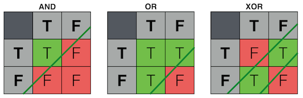
Here are the truth tables for two common logic gates:

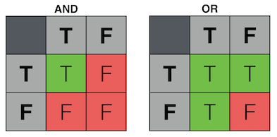
How could we implement these logical operations in electronic components?

AND Gate:

OR Gate:

* For an extended discussion of the analogy between electrical systems and artificial neural networks, see the "Common Analogies for Machine Learning" section of Machine Learning for Designers, published by O’Reilly Media, Inc., 2016.

Biological Analogy:

Biological neurons fire when there is sufficient activity in their inputs.

Loosely, we might think of this as:

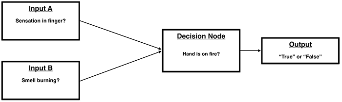
Of course, biological networks are complex (multilayered, so to speak).

The human brain definitely does not contain a single neuron that addresses the question of whether our hand is on fire.

In a more general (but still very loose) sense, it may be reasonable to say that we:

• monitor a group of input sensors
• weigh their relative importance
• determine the most appropriate behavior in response to these inputs

* For an extended discussion of the analogy between biological systems and artificial neural networks, see the "Common Analogies for Machine Learning" section of Machine Learning for Designers, published by O’Reilly Media, Inc., 2016.

(Prelude to) Training Perceptrons:

So far, we've looked at the feed-forward behavior of the Perceptron. But we have not yet considered how we train it to perform this behavior. In the above logic gate examples, how did we determine the proper signal voltages for each input? For these simple examples, we knew the desired behaviors and could therefore design for them explicitly. For more complex problems, however, it would be far more difficult to do so. Ideally, we would like the machine to implement the desired behavior on its own by learning from the examples that have been shown to it.

Mechanical Induction:

Excerpted from Machine Learning for Designers, published by O’Reilly Media, Inc., 2016.

Let's consider logic gates from an inductive point of view. In this case, we have a set of example inputs and outputs that exemplify a rule but do not know what the rule is. We wish to determine the nature of the rule using these examples.

Let’s again assume that the decision node’s output threshold is 1 volt. To reproduce the behavior of the AND gate by induction, we need to find voltage levels for the input signals that will produce the expected output for each pair of example inputs, telling us whether those inputs are included in the rule. The process of discovering the right combination of voltages can be seen as a kind of search problem.

One approach we might take is to choose random voltages for the input signals, use these to predict the output of each example, and compare these predictions to the given outputs. If the predictions match the correct outputs, then we have found good voltage levels. If not, we could choose new random voltages and start the process over. This process could then be repeated until the voltages of each input were weighted so that the system could consistently predict whether each input pair fits the rule.

In a simple system like this one, a guess-and-check approach may allow us to arrive at suitable voltages within a reasonable amount of time. But for a system that involves many more attributes, the number of possible combinations of signal voltages would be immense and we would be unlikely to guess suitable values efficiently. With each additional attribute, we would need to search for a needle in an increasingly large haystack.

Rather than guessing randomly and starting over when the results are not suitable, we could instead take an iterative approach. We could start with random values and check the output predictions they yield. But rather than starting over if the results are inaccurate, we could instead look at the extent and direction of that inaccuracy and try to incrementally adjust the voltages to produce more accurate results.

Biases:

Before we look more closely at the training process, let's consider a possible difficulty:

Recall the following step in the feed-forward process:

\(input_0 * weight_0\)
\(input_1 * weight_1\)

Given this, what would happen if:

\(input_0\) = 0
\(input_1\) = 0

In this case, it doesn't matter what the weights are!
The sum will always be zero.

To avoid this problem, we generally add an extra input to our Perceptron, called the bias input.
The bias input always has a value of 1 and is also weighted.

\(input_0\) = 0
\(input_1\) = 0
\(input_b\) = 1

\(input_0 * weight_0\) = 0
\(input_1 * weight_1\) = 0
\(input_b * weight_b\) = \(weight_b\)

In this case, the bias alone determines the output.
It biases the Perceptron's understanding of the line's position relative to the point [ 0, 0 ].

Implementation Detail:

You could implement biases in a few different ways:

• In your dataset ([ 1, -1 ] becomes [ 1, -1, 1 ], e.g.)
  • This option is most undesirable because it requires manually editing your dataset.
• When you run the Perceptron, you could append a 1 to the end of each input vector
  • This option is ok for small vectors, but is ultimately inefficient because it generally requires reallocating / copying lots of arrays.
• Store bias separate from other weights and add it in during the summing step.
  • This option is favorable and standard in many implementations.

Supervised Training Procedure:

We train the Perceptron by showing it examples for which we know the expected output, adjusting weights according to the incorrectness of the Perceptron's guessed output.

The Procedure:

1. Provide the Perceptron with inputs for which there are known outputs.
2. Ask the Perceptron to guess the outputs.
3. Compute the error.
4. Adjust all weights according to error.
5. Return to Step 1 and repeat.

Error Definition:

\( Error = {Output}_{Expected} - {Output}_{Guessed} \)

Error Delta:

\( \Delta{Weight} = Error * Input \)

Weight Update:

\( {Weight}_{New} = {Weight}_{Old} + \Delta{Weight} \)

Learning Rate:

We generally don't want to learn too much too quickly (from any one example).
So, we use a learning constant to limit the impact of our weight change:

\( {Weight}_{New} = {Weight}_{Old} + \Delta{Weight} * LearningConstant \)

where \(LearningConstant\) is a scalar value (presumably \(\lt\) 1).

Finding a good learning constant is relative to the dataset.
Experimentation is the best first approach, though it's possible to be more systematic.
We'll discuss this and related issues more in subsequent weeks.

Limitations of the Perceptron Model:

Unfortunately, Perceptrons are very limited in their learning capabilities. To better understand these limitations, let's consider a third form of logic gate: exclusive-or (XOR).

The behavior of an XOR gate could be worded as:
"The output will be activated if one or the other of the inputs is active, but not if both inputs are active."

Go back to the earlier electrical diagrams for AND and OR and see whether you can find input signal voltages that will enable the behavior of an XOR gate.

Start with the OR gate:

Again, we set the activation threshold to 1 volt and each of the input signals to 1 volt.

If only one of the inputs is active, then the sum of the input signals will equal 1 volt and the threshold will be reached.

If both inputs are active, the sum of the input signals will equal 2 volts, which exceeds the threshold and therefore activates the output.

Yet, to implement the XOR gate, we do not want the output to be activated if both inputs are active.

There is no way to achieve this behavior with a singular threshold value.

With AND and OR, a single cut (or "decision plane") separates the two output categories.

With XOR, we need two cuts. There is a mutual dependence between our inputs. We cannot simply look at each input dimension individually. If one is on, the other must be off.

For this reason, AND and OR are said to be linearly separable because their output space can be divided by a single line.

XOR, on the other hand, is not linearly seperable.

Interpretation:

Complex ideas often contain interrelated components.

Therefore, to learn complex ideas, we need some way of accounting for these kinds of interrelations.

Yet these interrelations may not be obvious simply by looking at the data itself.

What we need, in essence, is a strategy for allowing the machine to invent new dimensions whose express purpose is to characterize the interdependency between the "actual" data dimensions.

We'll talk more about these "hidden dimensions" in the coming weeks.

Discussion:

• What do these limitations tell us about the nature of learning?
• What conceptual alterations to the model might help to address these limitations?

Getting Started with Plotting in Python and Matplotlib

Importing Numpy library:

import numpy as np

Importing Pyplot library:

import matplotlib.pyplot as plt

Plot y-axis data:

# Note: x-axis is automatically generated as [ 0, 1, 2, 3 ]

plt.plot( [ 1, 4, 9, 16 ] )
plt.show()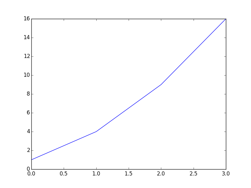

Plot x-axis and y-axis data:

plt.plot( [ 1, 2, 3, 4 ], [ 1, 4, 9, 16 ] )
plt.show()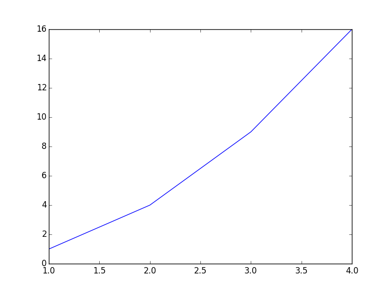

Plot x-axis and y-axis data with per-axis extents:

# Note: axis() formatted as [ xmin, xmax, ymin, ymax ]

plt.axis( [ 0, 6, 0, 50 ] )
plt.plot( [ 1, 2, 3, 4 ], [ 1, 4, 9, 16 ] )
plt.show()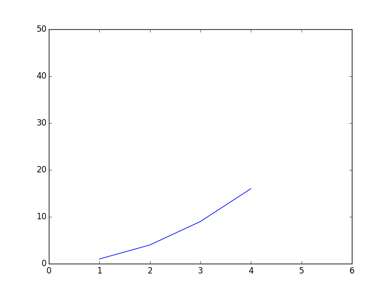

Customize axis labels:

plt.xlabel('X-AXIS DATA')
plt.ylabel('Y-AXIS DATA')
plt.plot( [ 1, 2, 3, 4 ], [ 1, 4, 9, 16 ] )
plt.show()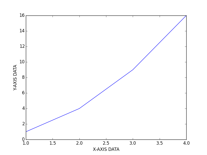

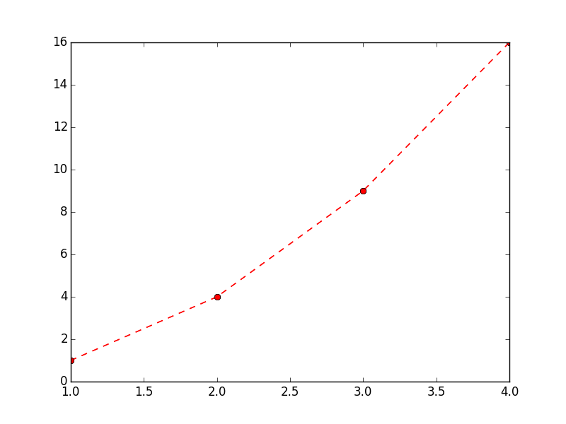
Customize plot stylization:

plt.plot( [ 1, 2, 3, 4 ], [ 1, 4, 9, 16 ], 'ro--')
plt.show() 

Additional documentation of stylization options can be found here: Pyplot Lines and Markers and Pyplot Line Properties

Plot functions:

def sigmoid(x):
    return 1.0 / ( 1.0 + np.exp( -x ) )

def dsigmoid(x):
    y = sigmoid( x )
    return y * ( 1.0 - y )

def tanh(x):
    return np.sinh( x ) / np.cosh( x )

def dtanh(x):
    return 1.0 - np.square( tanh( x ) )

xData = np.arange( -10.0, 10.0, 0.1 )
ySigm = sigmoid( xData )
ySigd = dsigmoid( xData )
yTanh = tanh( xData )
yTand = dtanh( xData )

plt.axis( [ -10.0, 10.0, -1.1, 1.1 ] )
plt.plot( xData, ySigm, 'r', xData, ySigd, 'r--' )
plt.plot( xData, yTanh, 'g', xData, yTand, 'g--' )
plt.show()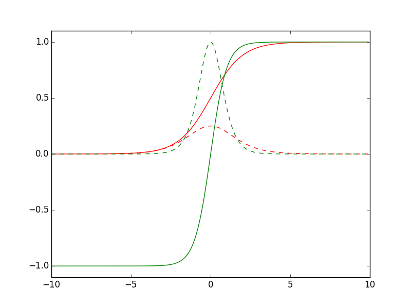 

Working with multiple figures and axes:

def f(t):
    return np.exp(-t) * np.cos(2*np.pi*t)

t1 = np.arange(0.0, 5.0, 0.1)
t2 = np.arange(0.0, 5.0, 0.02)

plt.figure(1)
plt.subplot(211)
plt.plot(t1, f(t1), 'bo', t2, f(t2), 'k')

plt.subplot(212)
plt.plot(t2, np.cos(2*np.pi*t2), 'r--')
plt.show()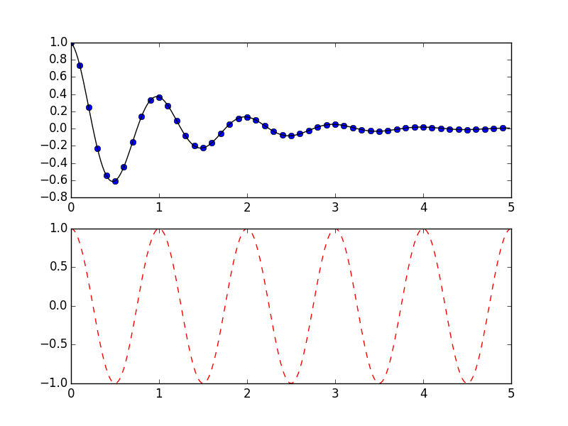

Working with text:

mu, sigma = 100, 15
x = mu + sigma * np.random.randn(10000)

# the histogram of the data
n, bins, patches = plt.hist(x, 50, normed=1, facecolor='g', alpha=0.75)

plt.xlabel('Smarts')
plt.ylabel('Probability')
plt.title('Histogram of IQ')
plt.text(60, .025, r'$\mu=100,\ \sigma=15$')
plt.axis([40, 160, 0, 0.03])
plt.grid(True)
plt.show()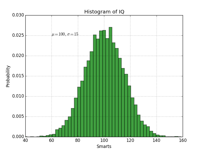

ax = plt.subplot(111)

t = np.arange(0.0, 5.0, 0.01)
s = np.cos(2*np.pi*t)
line, = plt.plot(t, s, lw=2)

plt.annotate('local max', xy=(2, 1), xytext=(3, 1.5),
            arrowprops=dict(facecolor='black', shrink=0.05),
            )

plt.ylim(-2,2)
plt.show()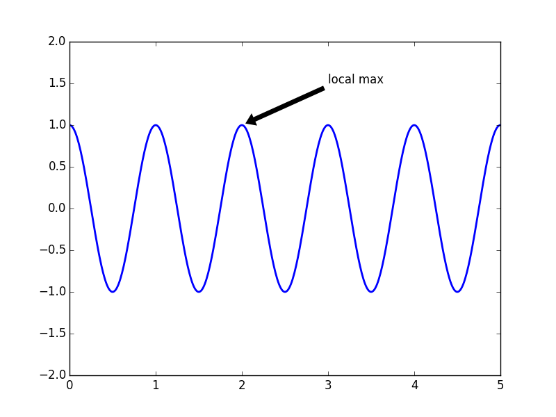

Plotting in 3D:

from mpl_toolkits.mplot3d import Axes3D
from matplotlib import cm
from matplotlib.ticker import LinearLocator, FormatStrFormatter

fig = plt.figure()
ax = fig.gca(projection='3d')
X = np.arange(-5, 5, 0.25)
Y = np.arange(-5, 5, 0.25)
X, Y = np.meshgrid(X, Y)
R = np.sqrt(X**2 + Y**2)
Z = np.sin(R)
surf = ax.plot_surface(X, Y, Z, rstride=1, cstride=1, cmap=cm.coolwarm,
                       linewidth=0, antialiased=False)
ax.set_zlim(-1.01, 1.01)

ax.zaxis.set_major_locator(LinearLocator(10))
ax.zaxis.set_major_formatter(FormatStrFormatter('%.02f'))

fig.colorbar(surf, shrink=0.5, aspect=5)

plt.show()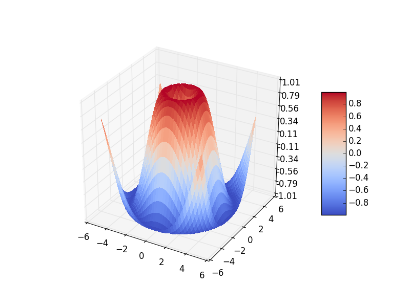

Additional Resources:

• Matplotlib Pyplot Tutorial
• Matplotlib Examples

Homework

Assignment:

• Implement a Perceptron in Python.

Readings:

• The Nature of Code by Daniel Shiffman, Chapter 10: "Neural Networks"
• Computational Neuroscience and Cognitive Modelling, Chapter 11: "An Introduction to Neural Networks"
• Primary Source: Learning Internal Representations by Error Propagation by David Rumelhart, Geoffrey Hinton and Ronald Williams