Taught by Patrick Hebron at ITP, Fall 2016
Homework Review
- Run-length encoding
- Discussion of readings
A Brief Tour of Fuzzy Logic
Excerpted from Machine Learning for Designers, published by O’Reilly Media, Inc., 2016.
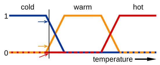
In our everyday communication, we generally use what logicians call fuzzy logic. This form of logic relates to approximate rather than exact reasoning. For example, we might identify an object as being “very small,” “slightly red,” or “pretty nearby.” These statements do not hold an exact meaning and are often context-dependent. When we say that a car is small, this implies a very different scale than when we say that a planet is small. Describing an object in these terms requires an auxiliary knowledge of the range of possible values that exists within a specific domain of meaning. If we had only seen one car ever, we would not be able to distinguish a small car from a large one. Even if we had seen a handful of cars, we could not say with great assurance that we knew the full range of possible car sizes. With sufficient experience, we could never be completely sure that we had seen the smallest and largest of all cars, but we could feel relatively certain that we had a good approximation of the range. Since the people around us will tend to have had relatively similar experiences of cars, we can meaningfully discuss them with one another in fuzzy terms.
Computers, however, have not traditionally had access to this sort of auxiliary knowledge. Instead, they have lived a life of experiential deprivation. As such, traditional computing platforms have been designed to operate on logical expressions that can be evaluated without the knowledge of any outside factor beyond those expressly provided to them. Though fuzzy logical expressions can be employed by traditional platforms through the programmer’s or user’s explicit delineation of a fuzzy term such as “very small,” these systems have generally been designed to deal with boolean logic (also called “binary logic”), in which every expression must ultimately evaluate to either true or false. One rationale for this approach is that boolean logic allows a computer program’s behavior to be defined as a finite set of concrete states, making it easier to build and test systems that will behave in a predictable manner and conform precisely to their programmer’s intentions.
Machine learning changes all this by providing mechanisms for imparting experiential knowledge upon computing systems. These technologies enable machines to deal with fuzzier and more complex or “human” concepts, but also bring an assortment of design challenges related to the sometimes problematic nature of working with imprecise terminology and unpredictable behavior.
Additional Resources:
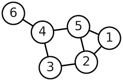
A Brief Tour of Graph Theory
In 1736, the mathematician Leonhard Euler published a paper on the Seven Bridges of Königsberg, which addressed the following question:
Königsberg is divided into four parts by the river Pregel, and connected by seven bridges. Is it possible to tour Königsberg along a path that crosses every bridge once, and at most once? You can start and finish wherever you want, not necessarily in the same place.
Euler looked at this problem from the perspective of how the edges, vertices and faces of a convex polyhedron relate to one another and in the process gave rise to a new study within mathematics, now called graph theory.
More generally, graph theory is the study of mathematical structures that can be used to model the pairwise relationships between objects. Graphs are comprised of vertices, which are connected to one another by edges.
In a directed graph, an edge represents a uni-directional relationship: a connection that flows from Vertex A to Vertex B, but not from Vertex B to Vertex A. In an undirected graph, an edge represents a bi-directional relationship: the connection flows from A to B as well as from B to A.
In a cyclic graph, the connections between vertices can form loops whereas in an acyclic graph they cannot.
These distinctions as well as others made by graph theory can be used to model an astoundingly wide variety of systems. It is used in physics, chemistry, biology, linguistics and many other fields. It is especially relevant to the field of computer science. Computer programs can be thought of as graphs that describe a flow of information through a series of operations. 2D and 3D design tools often represent users' projects as scenegraphs, which describe the hierarchical relationships between a series of geometric components.
Artificial neural networks are often thought about in these terms as well. Some neural architectures, such as many forms of classifiers, can be seen as directed acyclic graphs. Others, such as many forms of auto-encoders, can be represented as undirected graphs in which unencoded information can be passed in one direction to encode it while encoded information can be passed in the other direction to decode it. Recurrent neural networks are ones that allow loops (or "cycles") in their flow of information.
Machine learning draws upon metaphors from many other fields including neuroscience and thermodynamics. But graph theory has proven to provide a particularly good vocabulary for describing the kinds of nodal relationships that comprise the various forms of neural network models. Google's open-source machine learning library TensorFlow uses this mentality as its central organizing principle, as do several other popular machine learning systems. The "flow" in "TensorFlow" is a reference to the flow of information through a graph.
Though graph theory is a complex study in its own right, familiarity with its basic distinctions can be useful in understanding the composition of artificial neural networks.
Additional Resources:
Dimensions from 1 to N
- Euclidean Distance
- Abstract and Spatial Dimensions
- A Few Applications of Distance Metrics:
Linear Algebra Primer (Part 1)
Notation:
Scalar: x (lowercase, regular)
Vector: \(\mathbf{u}\) (lowercase, bold)
Vector: \(\overrightarrow{u}\) (lowercase, w/ arrow)
Summation: \(\sum\)
Product: \(\prod\)
Vector Definition:
Formal Definition:
An n-tuple of values (usually real numbers) where n is the "dimension" of the vector and can be any positive integer \(\ge\) 1.
A vector can be thought of as:
- a point in space
- a directed line segment with a magnitude and direction
Formatting:
- Vectors can be written in column form or row form
- Column form is conventional
- Vector elements are referenced by subscript
Column Vector:
\( \mathbf{x} = \begin{bmatrix} x_1 \\ \vdots \\ x_n \\ \end{bmatrix} \)
Row Vector:
\( \mathbf{x} = \begin{bmatrix} x_1 \cdots x_n \end{bmatrix} \)
Transpose Row Vector to Column Vector:
\( \begin{bmatrix} x_1 \cdots x_n \end{bmatrix}^\text{T} = \begin{bmatrix} x_1 \\ \vdots \\ x_n \\ \end{bmatrix} \)
Transpose Column Vector to Row Vector:
\( \begin{bmatrix} x_1 \\ \vdots \\ x_n \\ \end{bmatrix}^\text{T} = \begin{bmatrix} x_1 \cdots x_n \end{bmatrix} \)
Vector Properties:
- Vectors are commutative: ( \(\overrightarrow{u}\) + \(\overrightarrow{v}\) ) is equal to ( \(\overrightarrow{v}\) + \(\overrightarrow{u}\) )
- Vectors are associative: ( \(\overrightarrow{u}\) + ( \(\overrightarrow{v}\) + \(\overrightarrow{w}\) ) ) is equal to ( ( \(\overrightarrow{u}\) + \(\overrightarrow{v}\) ) + \(\overrightarrow{w}\) )
Working with Vectors in Python and Numpy:
Importing Numpy library:
import numpy as npArray Creation:
>>> np.array( [ 0, 2, 4, 6, 8 ] )
array([0, 2, 4, 6, 8])

>>> np.zeros( 5 )
array([ 0.,  0.,  0.,  0.,  0.])

>>> np.ones( 5 )
array([ 1.,  1.,  1.,  1.,  1.])

>>> np.zeros( ( 5, 1 ) )
array([[ 0.],
       [ 0.],
       [ 0.],
       [ 0.],
       [ 0.]])

>>> np.zeros( ( 1, 5 ) )
array([[ 0.,  0.,  0.,  0.,  0.]])

>>> np.arange( 5 )
array([0, 1, 2, 3, 4])

>>> np.arange( 0, 1, 0.1 )
array([ 0. ,  0.1,  0.2,  0.3,  0.4,  0.5,  0.6,  0.7,  0.8,  0.9])

>>> np.linspace( 0, 1, 5 )
array([ 0.  ,  0.25,  0.5 ,  0.75,  1.  ])

>>> np.random.random( 5 )
array([ 0.22035712,  0.89856076,  0.46510509,  0.36395359,  0.3459122 ])
Vector Addition:
Add corresponding elements. Result is a vector.
\[ \overrightarrow{z} = \overrightarrow{x} + \overrightarrow{y} = \begin{bmatrix} x_1 + y_1 \cdots x_n + y_n \end{bmatrix}^\text{T} \]
>>> x = np.array( [  1.0,  2.0,  3.0,  4.0,  5.0 ] )
>>> y = np.array( [ 10.0, 20.0, 30.0, 40.0, 50.0 ] )
>>> z = x + y
>>> z
array([ 11.,  22.,  33.,  44.,  55.])
Vector Subtraction:
Subtract corresponding elements. Result is a vector.
\[ \overrightarrow{z} = \overrightarrow{x} - \overrightarrow{y} = \begin{bmatrix} x_1 - y_1 \cdots x_n - y_n \end{bmatrix}^\text{T} \]
>>> x = np.array( [  1.0,  2.0,  3.0,  4.0,  5.0 ] )
>>> y = np.array( [ 10.0, 20.0, 30.0, 40.0, 50.0 ] )
>>> z = x - y
>>> z
array([ -9., -18., -27., -36., -45.])
Hadamard Product:
Multiply corresponding elements. Result is a vector.
\[ \overrightarrow{z} = \overrightarrow{x} \circ \overrightarrow{y} = \begin{bmatrix} x_1 y_1 \cdots x_n y_n \end{bmatrix}^\text{T} \]
>>> x = np.array( [  1.0,  2.0,  3.0,  4.0,  5.0 ] )
>>> y = np.array( [ 10.0, 20.0, 30.0, 40.0, 50.0 ] )
>>> z = x * y
>>> z
array([  10.,   40.,   90.,  160.,  250.])
Dot Product:
Multiply corresponding elements, then add products. Result is a scalar.
\[ a = \overrightarrow{x} \cdot \overrightarrow{y} = \sum_{i=1}^n x_i y_i \]
>>> x = np.array( [  1.0,  2.0,  3.0,  4.0,  5.0 ] )
>>> y = np.array( [ 10.0, 20.0, 30.0, 40.0, 50.0 ] )
>>> a = np.dot( x, y )
>>> a
550.0
Vector-Scalar Addition:
Add scalar to each element. Result is a vector.
\[ \overrightarrow{y} = \overrightarrow{x} + a = \begin{bmatrix} x_1 + a \cdots x_n + a \end{bmatrix}^\text{T} \]
>>> x = np.array( [  1.0,  2.0,  3.0,  4.0,  5.0 ] )
>>> a = 3.14
>>> y = x + a
>>> y
array([ 4.14,  5.14,  6.14,  7.14,  8.14])
Vector-Scalar Subtraction:
Subtract scalar from each element. Result is a vector.
\[ \overrightarrow{y} = \overrightarrow{x} - a = \begin{bmatrix} x_1 - a \cdots x_n - a \end{bmatrix}^\text{T} \]
>>> x = np.array( [  1.0,  2.0,  3.0,  4.0,  5.0 ] )
>>> a = 3.14
>>> y = x - a
>>> y
array([-2.14, -1.14, -0.14,  0.86,  1.86])
Vector-Scalar Multiplication:
Multiply each element by scalar. Result is a vector.
\[ \overrightarrow{y} = \overrightarrow{x} \ a = \begin{bmatrix} x_1 a \cdots x_n a \end{bmatrix}^\text{T} \]
>>> x = np.array( [  1.0,  2.0,  3.0,  4.0,  5.0 ] )
>>> a = 3.14
>>> y = x * a
>>> y
array([  3.14,   6.28,   9.42,  12.56,  15.7 ])
Vector-Scalar Division:
Divide each element by scalar. Result is a vector.
\[ \overrightarrow{y} = \frac{\overrightarrow{x}}{a} = \begin{bmatrix} \frac{x_1}{a} \cdots \frac{x_n}{a} \end{bmatrix}^\text{T} \]
>>> x = np.array( [  1.0,  2.0,  3.0,  4.0,  5.0 ] )
>>> a = 3.14
>>> y = x / a
>>> y
array([ 0.31847134,  0.63694268,  0.95541401,  1.27388535,  1.59235669])
Magnitude:
Compute vector length. Result is a scalar.
\[ a = || \overrightarrow{x} || = \sqrt{ x_1^2 + \cdots + x_n^2 } = \sqrt{ \overrightarrow{x} \cdot \overrightarrow{x} } \]
>>> x = np.array( [  1.0,  2.0,  3.0,  4.0,  5.0 ] )
>>> a = np.linalg.norm( x )
>>> a
7.416198487095663
Normalization:
Compute unit vector. Result is a vector.
\[ \hat{x} = \frac{\overrightarrow{x}}{|| \overrightarrow{x} ||} \]
>>> x = np.array( [  1.0,  2.0,  3.0,  4.0,  5.0 ] )
>>> a = np.linalg.norm( x )
>>> x = x / a
>>> x
array([ 0.13483997,  0.26967994,  0.40451992,  0.53935989,  0.67419986])
Additional Documentation:
Homework
Assignment:
- Implement a simple recommendation engine in Python. The Programming Collective Intelligence chapter listed below provides a complete solution, but please use this code only as a reference. Try implementing your recommendation engine with NumPy's vector tools.
- Spend some time experimenting with vectors in Python and NumPy. Try out the operations we've discussed: plug in different values and vector dimensions, consider the results, tweak the values and repeat. The more you play with these operations, the more intuitive they will become.
Readings:
- Programming Collective Intelligence by Toby Segaran, Chapter 2: "Making Recommendations" (Requires NYU ID for online access)
- Primary Source: The Perceptron: A Probabilistic Model for Information Storage and Organization in the Brain by Frank Rosenblatt