The workflow associated with the development of a machine learning system is somewhat different from that of a conventional computer program.
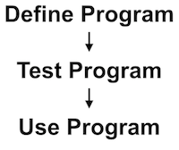
In a conventional software development process, the programmer dictates a series of concrete logical expressions that define each and every one of the program’s possible behaviors. The programmer then tests these logical expressions to ensure that they have been properly written and behave as expected. Once tested, the software can be deployed to and run by end-users.
Developing a machine learning system requires several additional stages:
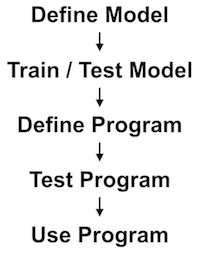
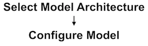
First, the developer must determine which machine learning algorithm or architecture is appropriate for the given task and either write the algorithm’s underlying mathematical operations or use an existing implementation provided by a machine learning library.
At this point, our machine learning system is more or less equivalent to a new-born baby. Its architecture makes it capable of learning complex patterns or ideas, but it has not yet had the experiences necessary to actualize this learning. In order to realize its potential, we must train the model on a set of example experiences that embody the patterns or ideas we wish for the system to learn.
In many cases, we must first customize the model for the specific learning task at hand. This generally involves choosing things like how many neurons will be used and selecting values for what are called the model’s hyperparameters or configuration variables. These values will be used to shape various aspects of the system’s learning process such as the extent to which the system will learn from any particular data sample shown to it.
Choosing good values for these hyperparameters is often highly contingent on the nature of the data and may require additional tweaking later in the development process. Once these hyperparameters have been defined, we can train the model on a dataset.
The training process tends to be highly computationally intensive due to the complex mathematical operations involved and therefore can take a great deal of time, sometimes many hours or even days.
During the training process, the developer uses various mechanisms to get a sense of whether the system is effectively learning about the data. These mechanisms will vary depending upon the type of machine learning algorithm that is being used.
In the case of supervised learning problem, since we know the expected output for any particular example input, we can ask the system to predict the output for a given input and compare this prediction to the expected output in order to arrive at an error rate. By watching this error rate change over the course of the training process, we can get a sense of whether the system is improving its ability to make correct predictions.
Generally speaking, we do not want to use the same set examples for training and testing our system. The reason for this is that we want to make sure that the system is learning the general concept we are demonstrating to it rather than simply memorizing the training examples.
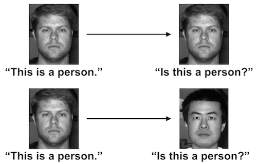
For example, if I showed you a single photograph of a person and told you, "this is a person," then later showed you the same image and asked you whether the image was of a person, I would have no way of knowing whether you truly understood the concept or had just memorized this one correlation.
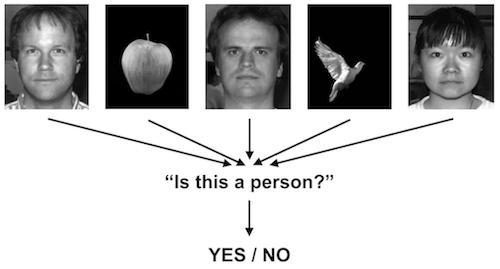
To get a better sense of your understanding, I should instead check whether you can correctly identify a person in a photo you have never seen before.
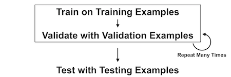
In most cases, this process of checking the system’s learning against examples that are not directly contained within the training set should be performed both during and after the training process.
The example used to check the system during the training process are often referred to as validation examples and those used after the training process are called testing examples.
After training and testing the system, if will often be necessary to make adjustments to the hyper parameters and other aspects of the model in order to improve the quality of learning in accordance with any limitations discovered through the testing process.
After making these changes, the system will need to be retrained.
Once the system has been trained and tested to show an acceptable learning level has been achieved, the machine learning system is now ready for use.
In most cases, the trained system will need to be embedded and used within a broader application.
At this point, we can think of the trained machine learning system as equivalent to a function within a conventional program. For example, we might embed an image recognizer within conventional programmatic logic such as this:
if( classifyImage( myImage ) == 'pizza' )
    return 'We have pizza!';
As with the development of a conventional program, the programmer defines a series of concrete logical expressions that define each and every one of the program’s possible behaviors, including ones that use the pre-trained machine learning system.
The programmer then tests these logical expressions to ensure that they have been properly written and behave as expected. In testing functionality that incorporates machine learning, the developer must be extra careful to ensure that the machine learning features are tested against a broad range of inputs that differ from the original training examples.
Once tested, the software can finally be deployed to and run by end-users.
Machine learning algorithms tend to require a great deal of computational resources due to the complex mathematical operations involved, which must generally be applied to many thousands or even millions of data samples during the training process.
For this reason, the average consumer laptop and even many of the machines used by professional programmers will not be powerful enough for use in the development of machine learning systems.

A computer's Central Processing Unit or CPU usually contains only one or a small handful of cores. Generally speaking, each core can only perform one mathematical operation at a time, which means that the typical CPU can only perform around 2 or 4 operations simultaneously.
Any additional operations needed to perform a particular calculation must wait in a queue until one of the cores finishes its current task and is ready for a new one. For even a relatively small machine learning training process, the number of necessary computations can add up quickly.
In a mathematical sense, however, many of these operations could be performed simultaneously. Therefore, it would be advantageous to use a processor that is specifically designed for performing many simultaneous calculations.
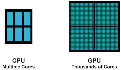
Graphics cards, also known as GPUs, were originally designed for performing the computationally intensive calculations associated with rendering 3D geometries in video games and other high performance graphics applications. GPUs employ an architecture quite different from those of CPUs and contain many hundreds or thousands of processing cores that work in parallel.
Though graphics and machine learning algorithms are different in some respects, they are generally built upon the same kinds of low-level mathematical operations. Therefore, it has become increasingly popular to use high-performance GPUs in machine learning work in order to accelerate computationally intensive training processes.

Some desktop and laptop machines designed especially for gamers come with high-performance GPUs that can be used for machine learning. Alternately, many machine learning developers rely upon servers that contain high powered GPUs, which they access remotely from their less powerful home or office computers.
The use of remote server allows developers to tap into extremely powerful machines that can greatly reduce the amount of time required to train a complex machine learning system.
Yet, this approach also introduces added complexity into the development process. Developers must coordinate and synchronize the versions of their software, any underlying toolkits used in their software and data across multiple systems and generally across networks.
To ensure the quality of learning in a training procedure, developers must pull back performance metrics data from the remote server. Any resulting changes to the model or its hyper parameters must be then be pushed back to the server.
Finding a suitable configuration for training a model on a particular dataset often involves a fair amount of experimentation, which means that this kind of synchronization needs to occur many times during the development process, adding significant complexity to the overall workflow.
Additionally, many machine learning tools have been developed primarily for use on Linux systems, though Mac and Windows versions are generally also available. As a result, developers must be conversant in multiple operating systems and feel comfortable moving fluidly between them many times a day.
A local gamer system removes some of this complexity, but is usually not as powerful as the kinds of machine learning accelerators available to server systems.
Despite the added complexity, these workflows can reduce the amount of time required to train a machine learning model by several orders of magnitude and have therefore become a standard component of working with machine learning systems.
Managing a machine learning workflow can be challenging at first. Fortunately, there are some great tools that can help with this process. Learning these tools may take a bit of time. But, once you're up and running, they will greatly reduce the amount of time you have to spend on the managerial and workflow aspects of your machine learning projects.
Docker is an open-source tool that automates the deployment of applications inside software containers.

As the Docker home page says, "Docker containers wrap up a piece of software in a complete filesystem that contains everything it needs to run: code, runtime, system tools, system libraries – anything you can install on a server. This guarantees that it will always run the same, regardless of the environment it is running in."
This can be very helpful in managing the development and deployment of software across multiple contributors, machines and operating systems.
A core element of Docker is what's called a dockerfile:
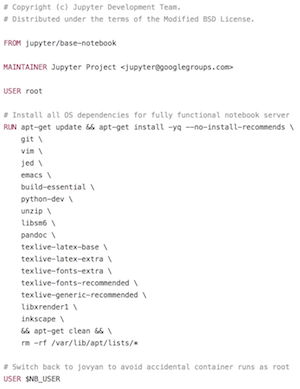
In essence, a docker file is a recipe for constructing a software environment that contains all of the underlying tools used within your project. For instance, a docker file might load tools like your favorite text editor, the python programming language, particular python libraries, git and so forth.
You can write a docker file from scratch. But, in many cases you'll be able to find a docker file that someone else has written and either use it directly or make minor modifications to it in order to incorporate all of the specific tools you need for your project. This can be shared with collaborators or used to spin up a server.
Though Docker has only been around for a few years, its ability to greatly simplify complex development and deployment processes has led it to quickly become a core component of many teams' software development workflows.
Machine learning tends to involve complex mathematical operations, which can be quite computationally intensive.
Though it is possible to write machine learning algorithms from scratch, it is often advantageous to use a machine learning library that offers optimized support for a wide range of mathematical operations as well as support for a range of computing platforms and accelerators such as high-performance GPUs.
TensorFlow is a numerical computation and machine learning library developed by Google and open-sourced in 2015. It has quickly become the most popular machine learning library.
It provides a flexible architecture that allows you to deploy computation to one or more CPUs or GPUs in a desktop, server, or mobile device — all using the same API.
TensorFlow can be used within several different programming languages including C, C++ and Java. However, TensorFlow was developed primarily for use with Python and currently offers the most features in that language.
The name TensorFlow may sound a bit exotic, but actually, it is quite descriptive:
The first part of the name, Tensor, refers to the mathematical concept of a Tensor and more broadly, to a field of mathematics called linear algebra, or the study of algebra in higher dimensions. Linear algebra allows us to apply algebraic operations to lists or grids of numbers.
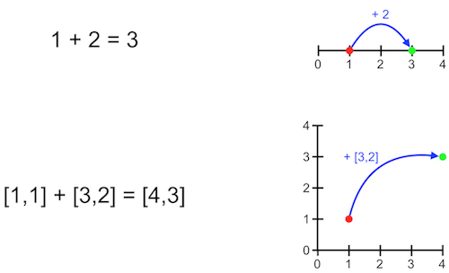
In ordinary algebra, we might add two numbers together in order to move from one point on a number line to another.
We can do something similar in higher dimensional space using linear algebra. For example, in a two-dimensional map, we might want to move from one point in a map to another.
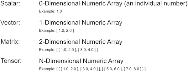
In linear algebra, the term ‘Scalar’ refers to an individual number. Or, to put it in a somewhat confusing way, a zero-dimensional array.
The term ‘Vector’ refers to a one-dimensional array.
The term ‘Matrix’ refers to a two-dimensional array.
The term ‘Tensor’ refers to an N-dimensional array, where N represents some specific number of dimensions.
Since scalars, vectors and matrices can all be represented as specializations of tensors, it makes sense to build a machine learning library around tensors as this allows us to represent all of these entities using the same basic data type, therefore providing the greatest flexibility to the programmer.
The second part of the name TensorFlow refers to the concept of a data flow graph and more broadly, to a field of mathematics called graph theory.
In general, graph theory is the study of abstract nodes and the connections between them. In the abstract, these nodes could represent many different kinds of entities. Graph theory itself deals with how these nodes are related to one another.
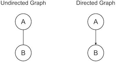
For example, in a directed graph, information can only flow between nodes in one direction whereas in an undirected graph, information can flow in either direction.
Amongst other things, this mechanism can be used to represent algebraic equations or the sequence of operations performed within a computer program.
Here is a simple algebraic formula depicted as a graph:
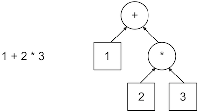
Notice that this graph explicitly represents the order of operations implied by the formula.
Computational graphs provide a powerful mental framework for thinking about and visualizing the complex sequences of operations applied by machine learning algorithms.
This approach also allows TensorFlow to analyze the structure of a particular graph and perform optimizations on it that will produce the same output in a more efficient manner.
Here is a complex neural network depicted as a graph:

We can imagine passing data into the input node of this graph and following it through a series of mathematical operations in order to arrive at some output.
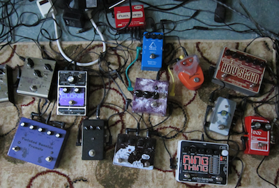
If you are a musician and have ever worked with signal processing pedals, you should feel right at home with this graph-based approach to computation.
The signal coming out of your guitar is equivalent to the graph’s input data.
This data moves through a wire to a pedal that processes or performs some computation on the signal before sending it along through another wire to the next pedal and eventually to the amplifier, which broadcasts the output.
By combining the concept of a Tensor — the most general form within linear algebra — with the broadly applicable concept of a computational or data flow graph, TensorFlow provides a powerful and highly flexible platform for working with machine learning systems.
Before we jump into TensorFlow, let’s review how we would write a simple arithmetic procedure in pure Python:
# Create input constants:
X = 2.0
Y = 3.0

# Perform addition:
Z = X + Y

# Print output:
print Z
When we run the above code, we get the following output:
5.0Let’s try to do the same thing using TensorFlow. First, we need to import the TensorFlow library into our Python environment:
# Import TensorFlow library:
import tensorflow as tf

# Print TensorFlow version, just for good measure:
print( 'TensorFlow Version: ' + tf.VERSION )
Let’s now write our first bit of TensorFlow code:
# Create input constants:
opX = tf.constant( 2.0 )
opY = tf.constant( 3.0 )

# Create addition operation:
opZ = tf.add( opX, opY )

# Print operation:
print opZ
When we run this code, the output may not be what we expect! Where is the resulting value? Rather than printing the number 5, we instead get a printout that seems to tell us the data type of the output:
Tensor("Add:0", shape=(), dtype=float32)This is because TensorFlow uses a somewhat different programming model from what we’re used to in pure Python. TensorFlow uses a graph-based approach to computation. In the code we’ve just written, we’ve defined the graph, but we haven’t actually executed it. To execute the graph and retrieve it’s output, we need to create what TensorFlow calls a session, which is an object that runs a graph and returns its output or outputs.
So, let’s again type out the operations that comprise our graph. This time, we'll also create a session and run the graph through it:
# Create input constants:
opX = tf.constant( 2.0 )
opY = tf.constant( 3.0 )

# Create addition operation:
opZ = tf.add( opX, opY )

# Create session:
with tf.Session() as sess:
    # Run session:
    Z = sess.run( opZ )
    # Print output:
    print Z
When we print the variable Z, we get back the numeric value we expected:
5.0For a simple arithmetic operation, this approach probably feels like overkill. But for more complex computations, it can be quite advantageous.
In the pure Python version of our code, the Python runtime executes each operation directly and immediately discards any intermediate information used in the process. For such a simple procedure, there isn’t really any intermediate information that’s worth holding onto.
By storing the graph rather than simply executing its component operations, TensorFlow can analyze and optimize the graph and do things like compute an operation’s derivative. This would not be possible if we only kept the result of an operation and not a representation of the operation itself.
So while TensorFlow’s graph-based model adds a bit of initial complexity to our workflow, it will greatly simplify more complex tasks as we dive deeper.
First, we need to import the TensorFlow library into our Python environment:
# Import TensorFlow library:
import tensorflow as tf
Let's review the basic use of constants:
# Create constants:
X = tf.constant( 2.0 )
Y = tf.constant( 3.0 )

# Create addition operation:
Z = tf.add( X, Y )

# Create session:
with tf.Session() as sess:
    # Run session:
    output = sess.run( Z )
    # Print output:
    print output
Our use of the operation tf.constant assumes that each time we run a session on the graph, we will want the same values to be associated with X and Y.
In many cases, however, we want to define a graph in a more generic manner and only assign the actual input values when we run a session on the graph.
Imagine you were building a facial recognition system. You wouldn’t want to pre-load the system with a single image. You would want to be able to load different images each time you ran the system.
The operation tf.placeholder allows us to do just that:
# Create placeholders:
X = tf.placeholder( tf.float32 )
Y = tf.placeholder( tf.float32 )

# Create addition operation:
Z = tf.add( X, Y )

# Create session:
with tf.Session() as sess:
    # Run session and print output:
    print sess.run( Z, feed_dict={ X: 2.0, Y: 3.0 } )
    # Run session and print output (with different input values):
    print sess.run( Z, feed_dict={ X: 4.0, Y: 5.0 } )
When we run a session on the operation, we must now feed it specific values for each of our placeholders. We do this by adding a second parameter to our session runner call. We create a dictionary called "feed_dict" and then associate each of our placeholders with an actual value. Now, we can run the same graph multiple times, plugging different values into X and Y each time we run it.
So far, we’ve been running our graphs on scalars or individual numbers. In TensorFlow, these scalars are treated as zero-dimensional Tensors. Most often, though, we’ll be running our graphs on higher dimensional Tensors:
# Create matrix constants:
X = tf.constant( [ [ 2.0, -4.0, 6.0 ], [ 5.0, 7.0, -3.0 ] ] )
Y = tf.constant( [ [ 8.0, -5.0 ], [ 9.0, 3.0 ], [ -1.0, 4.0 ] ] )

# Create matrix multiplication operation:
Z = tf.matmul( X, Y )

# Create session:
with tf.Session() as sess:
    # Run session:
    output = sess.run( Z )
    # Print output:
print outputFirst, we need to import the TensorFlow library into our Python environment. For this example, we're going to display an image within our Jupyter notebook, so we'll import the matplotlib and numpy libraries to help with that:
# Import TensorFlow library:
import tensorflow as tf

# Import matplotlib and numpy libraries (used to show image):
from matplotlib.pyplot import imshow
import numpy as np
Let’s look at two approaches to loading data into TensorFlow.
In cases where we need to pass a small amount of data to TensorFlow (a tensor containing just a few numbers, for instance) we can simply construct a pure Python list and use it to fill a tf.constant or feed a tf.placeholder:
# Create python list constants:
constantX       = [  1.0,  2.0,  3.0 ]
constantY       = [ 10.0, 20.0, 30.0 ]

# Create addition operation (for constants):
addConstants    = tf.add( constantX, constantY )

# Create session:
with tf.Session() as sess:
    # Run session on constants and print output:
    print sess.run( addConstants )

# Create placeholders:
placeholderX    = tf.placeholder( tf.float32 )
placeholderY    = tf.placeholder( tf.float32 )

# Create addition operation (for placeholders):
addPlaceholders = tf.add( placeholderX, placeholderY )

# Create session:
with tf.Session() as sess:
     # Run session on placeholders and print output:
    print sess.run( addPlaceholders, feed_dict={ placeholderX: constantX, placeholderY: constantY } )
This approach can be quite handy when working with relatively small data elements that can be reasonably embedded within our Python code. But, in most machine learning applications, the data we’ll be using will be much larger. We certainly wouldn’t want to type out each pixel value of an image by hand!
In many cases, we’ll want to load data from a file:
# Define file-reader function:
def read_file(filepath):
    file_queue  = tf.train.string_input_producer( [ filepath ] )
    file_reader = tf.WholeFileReader()
    _, contents = file_reader.read( file_queue )
    return contents

# Create PNG image loader operation:
load_op = tf.image.decode_png( read_file( 'data/tf.png' ) )

# Create JPG image loader operation:
# load_op = tf.image.decode_jpg( read_file( 'data/myimage.jpg' ) )

# Create session:
with tf.Session() as sess:
    # Initialize global variables:
    sess.run( tf.global_variables_initializer() )

    # Start queue coordinator:
    coord   = tf.train.Coordinator()
    threads = tf.train.start_queue_runners( coord=coord )

    # Run session on image loader op:
    image = sess.run( load_op )

    # Terminate queue coordinator:
    coord.request_stop()
    coord.join( threads )

    # Show image:
imshow( np.asarray( image ) )Now that we have a basic sense of TensorFlow’s workflow, let’s build and train our very first neural network. Recall that machine learning provides techniques for automating inductive processes. In inductive reasoning, we start from a set of examples of some phenomenon and use these to try to produce a general theory or formula that describes or approximates the phenomenon as a whole.
In our case, the formula we’ll be trying to approximate is the equation for a straight line in two dimensions.
Drawing upon outside knowledge, we already know that the equation we’re trying to approximate is as follows:
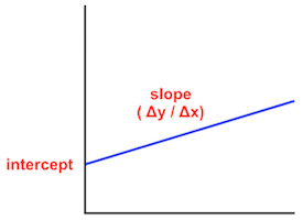
y = slope * x + interceptwhere the slope of a line is the ratio of its change in the y-axis divided by its change in the x-axis and the intercept is location where the line crosses the y-axis.
But our neural network will not have access to this formula. Instead, we will choose particular values for the slope and intercept of a particular line and then generate a set of example (X,Y) coordinates that fall on or near this line.
These example coordinates will be used to train the neural network, so that hopefully we end up with a neural approximation of our line that can be used to predict the Y value for any particular X value we feed it.
First, we need to import the necessary libraries into our Python environment:
# Import TensorFlow library:
import tensorflow as tf

# Import Numpy library:
import numpy as np

# Import Matplotlib pyplot library:
import matplotlib.pyplot as plt
Next, we’ll choose specific values for the slope and intercept of a particular line, define a few parameters that will be used in the training of our neural network and create our training data:
# Line equation:
# y = slope * x + intercept

# Set target slope and intercept:
target_slope     =   12.0
target_intercept =    7.0

# Set training parameters:
num_examples     =   25
num_epochs       = 1000
learning_rate    =    0.01

# Create random noise:
noise_level      = 5.0
noise            = np.random.uniform( -noise_level, noise_level, size = num_examples )

# Create training data:
trainX           = np.linspace( 0.0, 10.0, num = num_examples )
trainY           = target_slope * trainX + target_intercept + noise
Now that we have our data ready, we can build the neural network:
# Create input placeholders:
X                = tf.placeholder( tf.float32 )
Y                = tf.placeholder( tf.float32 )

# Create weight and bias variables:
W                = tf.Variable( np.random.randn(), name="weight" )
b                = tf.Variable( np.random.randn(), name="bias" )

# Create prediction operation:
predict          = tf.add( tf.multiply( X, W ), b )

# Create mean squared error (MSE) cost function:
cost             = tf.reduce_sum( tf.pow( predict - Y, 2.0 ) ) * ( 1.0 / num_examples )

# Create gradient descent optimizer:
optimizer        = tf.train.GradientDescentOptimizer( learning_rate ).minimize( cost )
To train the network, we will pass X values in from our training data and ask the network to use this prediction operation to predict the corresponding Y value. Since the slope and intercept values are initially random, these predictions will initially be quite incorrect.
To measure the incorrectness of its predictions, we use a mean squared error cost function. You may notice that this equation bears a striking resemblance to the Pythagorean formula. In essence, this describes how far a given predicted Y value is from the actual Y value in the training example.
Our neural network’s goal in the training process will be to reduce this error as much as possible so that the predicted Y values are very similar to the actual Y values. To do so, the network will need to make adjustments to the slope and intercept values that yield more accurate predictions.
One way to think about this process is to imagine that you’re standing at the top of a hill and want to get to the bottom of it. Standing at the top, you look around you and take one step in whatever direction lowers your elevation the most. When you get there, you again look around and take another step in whatever direction takes you the furthest downhill. You repeat this process until (hopefully) you are at the bottom of the hill.
In our case, the hill is our error rate and taking a step is equivalent to changing the slope and intercept values in one direction or another. This process (more or less) is called gradient descent. The gradient is the curvature of the hill, which we want to discover so that we can figure out how to descend along the hill as quickly as possible. To do this mathematically involves some calculus.
Fortunately for us, TensorFlow provides a feature that does this automatically. To use it, we define a gradient descent optimizer, pass it our chosen learning rate and cost function and it will do the rest.
With the operations now defined, we are finally ready to train our neural network. We'll also use Matplotlib to plot our predictions in order to get a better sense of how the training is progressing:
# Create session:
with tf.Session() as sess:
    # Initialize global variables:
    sess.run( tf.global_variables_initializer() )

    # Iterate over each training epoch:
    for epoch in range( num_epochs ):
        # Iterate over each training pair:
        for ( x, y ) in zip( trainX, trainY ):
            # Run optimizer on training pair:
            sess.run( optimizer, feed_dict = { X: x, Y: y } )

        # Print stats:
        if ( epoch + 1 ) % 25 == 0:
            curr_cost = sess.run( cost, feed_dict = { X: trainX, Y: trainY } )
            curr_W    = sess.run( W )
            curr_b    = sess.run( b )
            print "Epoch:", '%04d' % ( epoch + 1 ), \
                  "cost=", "{:.4f}".format( curr_cost ), \
                  "W=", "{:.4f}".format( curr_W ), \
                  "b=", "{:.4f}".format( curr_b )

    # Plot training data:
    plt.plot( trainX, trainY, 'ro', label = 'Data' )
    # Plot predictions:
    plt.plot( trainX, trainX * sess.run( W ) + sess.run( b ), label = 'Prediction' )
    # Plot legend:
    plt.legend()
    # Show plot:
plt.show()After training a neural network, we need some way to save the model so that later we can restore the model and either continue to train it or use it to make predictions.
Let’s take a look at how to save and restore our linear regression model in TensorFlow.
# Import TensorFlow library:
import tensorflow as tf

# Import Numpy library:
import numpy as np

# Import Matplotlib pyplot library:
import matplotlib.pyplot as plt
To prepare our code for saving and restoring models, the first thing we’ll want to do is specify a file path where the model will be saved. Here, we've added a "save_path" variable that represents the file path we’ll use to save the model. This path ends with the ".ckpt" extension, which stands for checkpoint, a common naming convention for saved machine learning models.
# Line equation:
# y = slope * x + intercept

# Set target slope and intercept:
target_slope     =   12.0
target_intercept =    7.0

# Set training parameters:
num_examples     =   25
num_epochs       = 1000
learning_rate    =    0.01

# Create random noise:
noise_level      = 5.0
noise            = np.random.uniform( -noise_level, noise_level, size = num_examples )

# Create training data:
trainX           = np.linspace( 0.0, 10.0, num = num_examples )
trainY           = target_slope * trainX + target_intercept + noise

# Set save path:
save_path        = "data/linear_regression_model.ckpt"
We will then define the graph as we did before:
# Create input placeholders:
X                = tf.placeholder( tf.float32 )
Y                = tf.placeholder( tf.float32 )

# Create weight and bias variables:
W                = tf.Variable( np.random.randn(), name="weight" )
b                = tf.Variable( np.random.randn(), name="bias" )

# Create prediction operation:
predict          = tf.add( tf.multiply( X, W ), b )

# Create mean squared error (MSE) cost function:
cost             = tf.reduce_sum( tf.pow( predict - Y, 2.0 ) ) * ( 1.0 / num_examples )

# Create gradient descent optimizer:
optimizer        = tf.train.GradientDescentOptimizer( learning_rate ).minimize( cost )
Just before opening the session, we’ll add a TensorFlow saver operation, which will be used to save the model. Within the session, we’ll train the model again as we did before. At the very end of the session code, we will pass the session and file path to the saver operation in order to save the model to file:
# Create saver op to save and restore all variables:
saver = tf.train.Saver()

# Create session:
with tf.Session() as sess:
    # Initialize global variables:
    sess.run( tf.global_variables_initializer() )

    # Iterate over each training epoch:
    for epoch in range( num_epochs ):
        # Iterate over each training pair:
        for ( x, y ) in zip( trainX, trainY ):
            # Run optimizer on training pair:
            sess.run( optimizer, feed_dict = { X: x, Y: y } )

        # Print stats:
        if ( epoch + 1 ) % 25 == 0:
            curr_cost = sess.run( cost, feed_dict = { X: trainX, Y: trainY } )
            curr_W    = sess.run( W )
            curr_b    = sess.run( b )
            print "Epoch:", '%04d' % ( epoch + 1 ), \
                  "cost=", "{:.4f}".format( curr_cost ), \
                  "W=", "{:.4f}".format( curr_W ), \
                  "b=", "{:.4f}".format( curr_b )

    # Plot training data:
    plt.plot( trainX, trainY, 'ro', label = 'Data' )
    # Plot predictions:
    plt.plot( trainX, trainX * sess.run( W ) + sess.run( b ), label = 'Prediction' )
    # Plot legend:
    plt.legend()
    # Show plot:
    plt.show()

    # Save model:
    model_path = saver.save( sess, save_path )
    print( "Model saved to: %s" % model_path )
We'll now pretend a few days have passed and we want to restore our saved model and use it to make predictions. We create a new session and run the global values initializer as we did before and then call the saver's restore function and pass it our new session and the model file path:
# Create new session:
with tf.Session() as sess:
    # Initialize global variables:
    sess.run( tf.global_variables_initializer() )

    # Restore model:
    saver.restore( sess, save_path )
    print( "Model restored from: %s" % save_path )

    # Plot training data:
    plt.plot( trainX, trainY, 'ro', label = 'Data' )
    # Plot predictions:
    plt.plot( trainX, trainX * sess.run( W ) + sess.run( b ), label = 'Prediction' )
    # Plot legend:
    plt.legend()
    # Show plot:
    plt.show()