Based on CSC321: Neural Networks, by Geoffrey Hinton.
Relation to Perceptrons
Multilayer Perceptrons do not use the Perceptron learning algorithm. As Geoff Hinton says, they never should have been called Multilayer Perceptrons because the Perceptron learning algorithm cannot be generalized to hidden layers.
Perceptron convergence works by ensuring that every time the weights change, they get closer to every "generously feasible" set of weights.
This type of guarantee cannot be extended to more complex networks in which the average of two good solutions may be a bad solution.
So, "multi-layer" networks do not use the Perceptron learning algorithm.
Demonstrating Progress
Instead of showing that the weights are getting closer to a good set of weights,
show that the actual output values are getting closer to the target values.
This can be true even for non-convex problems where lots of different sets of weights could work well and averaging two good sets of weights may give a bad set of weights. It is not true of Perceptron learning.
Moving Beyond the Perceptron's Limitations
Neural networks without any hidden units are very limited in what they can model.
Adding a layer of hand-picked features to Perceptrons makes them much more powerful.
But it is difficult to design good features, especially for a complex problem!
We want to find good features without requiring any human insights into the task. We also want to avoid repeated trial-and-error.
We need to automate the process of designing features for a specific task and seeing how well they work.
A First Attempt Using an Evolutionary Mindset
Looking to the natural world for inspiration is often a good starting point.
Evolution provides an obvious point of entry to the problem of iteratively optimizing a set of weights in order to address a specific task.
As a basic sketch, we might consider a procedure like this:
Unfortunately, this approach is extremely inefficient.
To check whether a single weight change improves the system's performance, we need to compute at the predicted output for a large number of training examples.
Towards the end of the training process, large weight changes will usually make things worse because the weights need to have the right relative values to one another. One way to understand this problem is to imagine trying to solve a Rubik's Cube by getting a single face to be all one color, then moving to the next face. You end up undoing your earlier work!
Evolution is clearly a powerful mechanism in nature. But it also requires an immense amount of time. Ideally, we can find a more efficient approach!
We could try randomly changing all of the weights at the same time.
But this isn't any better because we would need to perform many trials on each training example in order to distinguish the impact on one weight from the noise created by changing all of the other weights. (Again, think of the Rubik's cube)
A better approach would be to make random changes to the hidden units' activities.
If we know how we want to change the hidden unit's activities for a specific training example, we can figure out how to change the weights accordingly.
Backpropagation Conceptual Overview
We don't know exactly what we want the hidden units to do. But we can compute the rate of change in the prediction error as we change a hidden activity.
Rather than using the desired activities to train the hidden units, we will instead use error derivatives with respect to the hidden activities.
Each hidden activity will impact numerous output units and can therefore have many different effects upon the overall error. These effects must be combined.
We can efficiently compute error derivatives for all hidden units simultaneously.
Backpropagation Overview for a Single Training Example
Let's now look at how to extend this to a full training procedure:
The Delta Rule
\( \begin{align} \Delta{w} & = w - w_{old} \\ \\ & = - LearningConstant \frac{\partial{E}}{\partial{w}} \\ \\ & = (LearningConstant)(y_{target}-y)(x) \\ \\ \end{align} \)
or...
\( w = w_{old} + (LearningConstant)(y_{target}-y)(x) \)
The Delta Rule is similar to the Perceptron Learning Rule, but differs in the following ways:
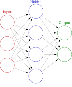
Multilayer Perceptron Architecture
Each node in the hidden layer is a function of the nodes in the previous layer.
The output node is a function of the nodes in the hidden layer.
Multilayer Perceptron Training Procedure
There are many possible ways of organizing a Multilayer Perceptron implementation. The approach below attempts modularize the components while hopefully keeping the code relatively easy to read. One of the more confusing aspects of implementing an MLP is keeping track of the signal array indices as we move forwards and backwards through the layers. This could be aided by moving more of the component functionality into the class representing an individual layer within the network.
import numpy as np

# Activation function definitions:

def sigmoid_fn(x):
    return 1.0 / ( 1.0 + np.exp( -x ) )

def sigmoid_dfn(x):
    y = sigmoid_fn( x )
    return y * ( 1.0 - y )

def tanh_fn(x):
    return np.sinh( x ) / np.cosh( x )

def tanh_dfn(x):
    return 1.0 - np.power( tanh_fn( x ), 2.0 )

# MLP Layer Class:

class MlpLayer:
    def __init__(self,input_size,output_size):
        self.weights = np.random.rand( output_size, input_size ) * 2.0 - 1.0
        self.bias    = np.zeros( ( output_size, 1 ) )

# MLP Class:

class Mlp:
    def __init__(self,layer_sizes,activation_fn_name):
        # Create layers:
        self.layers = []
        for i in range( len( layer_sizes ) - 1 ):
            self.layers.append( MlpLayer( layer_sizes[ i ], layer_sizes[ i + 1 ] ) )
        # Set activation function:
        if activation_fn_name == "tanh":
            self.activation_fn  = tanh_fn
            self.activation_dfn = tanh_dfn
        else:
            self.activation_fn  = sigmoid_fn
            self.activation_dfn = sigmoid_dfn

    def predictSignal(self,input):
        # Setup signals:
        activations = [ input ]
        outputs     = [ input ]
        # Feed forward through layers:
        for i in range( 1, len( self.layers ) + 1 ):
            # Compute activations:
            curr_act = np.dot( self.layers[ i - 1 ].weights, outputs[ i - 1 ] ) + self.layers[ i - 1 ].bias
            # Append current signals:
            activations.append( curr_act )
            outputs.append( self.activation_fn( curr_act ) )
        # Return signals:
        return activations, outputs

    def predict(self,input):
        # Feed forward:
        activations, outputs = self.predictSignal( input )
        # Return final layer output:
        return outputs[ -1 ]

    def trainEpoch(self,input,target,learn_rate):
        num_outdims  = target.shape[ 0 ]
        num_examples = target.shape[ 1 ]
        # Feed forward:
        activations, outputs = self.predictSignal( input )
        # Setup deltas:
        deltas = []
        count  = len( self.layers )
        # Back propagate from final outputs:
        deltas.append( self.activation_dfn( activations[ count ] ) * ( outputs[ count ] - target ) )
        # Back propagate remaining layers:
        for i in range( count - 1, 0, -1 ):
            deltas.append( self.activation_dfn( activations[ i ] ) * np.dot( self.layers[ i ].weights.T, deltas[ -1 ] ) )
        # Compute batch multiplier:
        batch_mult = learn_rate * ( 1.0 / float( num_examples ) )
        # Apply deltas:
        for i in range( count ):
            self.layers[ i ].weights -= batch_mult * np.dot( deltas[ count - i - 1 ], outputs[ i ].T )
            self.layers[ i ].bias    -= batch_mult * np.expand_dims( np.sum( deltas[ count - i - 1 ], axis=1 ), axis=1 )
        # Return error rate:
        return ( np.sum( np.absolute( target - outputs[ -1 ] ) ) / num_examples / num_outdims )

    def train(self,input,target,learn_rate,epochs,batch_size = 10,report_freq = 10):
        num_examples = target.shape[ 1 ]
        # Iterate over each training epoch:
        for epoch in range( epochs ):
            error = 0.0
            # Iterate over each training batch:
            for start in range( 0, num_examples, batch_size ):
                # Compute batch stop index:
                stop = min( start + batch_size, num_examples )
                # Perform training epoch on batch:
                batch_error = self.trainEpoch( input[ :, start:stop ], target[ :, start:stop ], learn_rate )
                # Add scaled batch error to total error:
                error += batch_error * ( float( stop - start ) / float( num_examples ) )
            # Report error, if applicable:
            if epoch % report_freq == 0:
                # Print report:
                print "Epoch: %d\nError: %f\n" % ( epoch, error )
Take a look at the full Multilayer Perceptron implementation, which also includes a Matplotlib visualizer for tracking the training process:
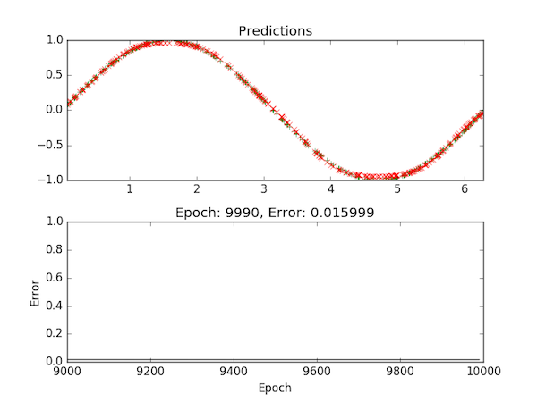
You can find the full Updated Multilayer Perceptron implementation code in the class repo.
Supervised learning is useful for problems in which we have a set of example inputs and corresponding outputs that implicitly demonstrate some function or behavior that is not explicitly known to us.
Supervised learning problems generally fall into one of two categories: regression problems and classification problems.
In a regression problem, the outputs relate to a real-valued number. For example, based on a set of financial metrics and past performance data, we might try to guess the future price of a particular stock.
In a classification problem, the outputs relate to a set of discrete categories. For example, we might have an image of a handwritten character and want to determine which of 26 possible letters it represents.
A general-purpose supervised learning system should be capable of learning about a regression or a classification problem. What the system learns is entirely dependent upon the data you provide to it.
For any particular learning problem and set of example data, there are often numerous ways in which the data could be arranged and presented to the system. The structure and formatting of this data will play a key role in the system's ability to learn from the data.
As we work towards applying supervised learning to real-world problems, let's take a closer look at the nature of regression and classification problems and then consider some encoding mechanisms for making data more comprehendible to a learning machine.
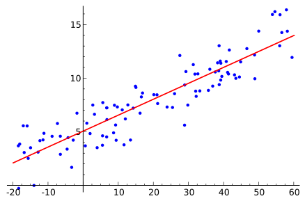
In statistics, regression is the process of trying to find a simple mathematical function that fits a set of data relatively well.
Why relatively well? Why not perfectly?!
Real-world data is almost never perfect. Even when the behavior of a particular system is predominantly governed by one specific law, there are usually several other forces that have at least some impact on the system's behavior.
For example, we could use a handful of well-defined formulae to describe the behavior of a simple physical system such as a bouncing ball. But, in practice, it would be impossible to account for every single force acting upon an actual bouncing ball. Perhaps we have forgotten to model the slight wind blowing through the room, causing the physical ball's motion to deviate slightly from its expected trajectory.
Very often, we don't care about these slight imprecisions or subtle auxiliary forces - we are looking for a good general approximation of the dominant forces.
This brings us to a problem-solving principle known as Occam's razor, which is very closely related to regression problems.
The principle of Occam's razor is generally stated in the following way:
Among competing hypotheses, the one with the fewest assumptions should be selected.
Of course, some phenomena are very complicated and the simplest hypothesis is still a complicated function. And, of course, it is possible to produce an overly-simplistic hypothesis that does not adequately describe a given phenomenon.
Nonetheless, to understand the world we sometimes need to ignore the minute details or risk getting lost in them.
Within the field of statistics, there are multiple approaches to performing regression without machine learning. In general, these approaches fall into two basic categories:
Linear Regression techniques try to fit data to a straight line.
Non-Linear Regression techniques try to fit data to a curve such as a polynomial expression.
As a machine learning problem, we do not need to make the distinction between linear and non-linear models. Instead, we will try to induce a good approximation of the function that is implied by the data.
While a statistical approach may yield a concrete description such as a straight-line equation, the neural network's implicit representation of the function will look nothing like an algebraic formula. Instead, the function is stored as a distributed representation that can simulate the behavior of the algebraic formula.
In applying machine learning to regression problems, there are several things we need to watch out for to ensure that the system produces a good general approximation of the data. Namely, it is possible to produce an approximation that conforms too literally to the training examples and will not perform well with other similar examples that were not expressly contained within the training set. This is called overfitting. It is also possible to produce an under-specified generalization that does not sufficiently conform to the data. This is called under-fitting. We will discuss these more in a section below.
Some machine learning problems require the prediction of a discrete categorical output instead of a real-valued output.
For some supervised learning problems, it may be equally reasonable to frame the problem in terms of classification or regression. For example, in making stock market predictions, we could try to predict the future price of a stock or alternately try to make categorical predictions of whether to "buy," "hold" or "sell."
In some cases, it may be reasonable to consider an intermediate point between two discrete categories. For example, if we had "hot" and "cold" categories, we could imagine various stopping points between these extremes, such as "warm" and "cool."
In other cases, intermediate points may not be conceptually meaningful. For example, if we had "tree" and "human" categories, what would the halfway point between these two extremes represent?
In order to train a neural network on categorical information, we need some way of representing the categories numerically.
For example:
Textual Representations: { "Buy", "Hold", "Sell" }
Indexical Representations: { 0, 1, 2 }
We could treat this data a single dimension, similarly to real-valued data, and try to fit the data into the numeric range of [ 0 .. 2 ]. We would then need to think about rounding - what to do with an output such as 1.5.
If we have hundreds of categories ( e.g., [ 0 .. 500 ] ) and compress this information into a single dimension for a Multilayer Perceptron's sigmoid range of [ 0 .. 1 ], when we re-expand the MLP's output to [ 0 .. 500 ], there is likely to be a significant loss of precision.
To get around this potential loss of precision, we might consider using a numerical encoding scheme that utilizes a greater number of dimensions to represent the categories.
At first, we might consider something along the lines of a binary representation of a category index. For example, category "5" could be encoded as "00000101." But here, we need to consider what the neural network is actually learning. To correctly predict outputs using this encoding scheme, the neural network would, in a sense, need to learn how binary encodings work in addition to learning about whatever classification task you're trying to perform.
Since we will generally want to think of each category as a unique entity within a classification problem, it might make sense to give each category its own dimension!
In a one-hot encoding, each category is given its own dimension. The value associated with the active dimension (aka category) is set to 1. The value associated with each other dimension is set to 0.
For example:
Textual Representations: { "Buy", "Hold", "Sell" }
One-Hot Representations: { [ 1, 0, 0 ], [ 0, 1, 0 ], [ 0, 0, 1 ] }
A one-cold encoding is the opposite - the active dimension is set to 0 and then inactive dimensions are set to 1.
One-hot encodings are more commonly used than one-cold encodings, but they represent the same basic idea.
In some cases, the data we wish to learn about represents sequential or temporal events.
In recent years, recurrent neural networks have shown themselves to be especially good at dealing with sequential data. We will discuss recurrent networks later in the semester.
It is also possible to apply a standard supervised learning system to a sequence learning problem by structuring the data in a manner that makes its sequential nature accessible to the learner.
Let's say we have a dataset that contains a sequence of events and we want to train the system to predict the next event:
{ Event 0, Event 1, Event 2, Event 3, ... }
To train a supervised system to perform this task, we can organize our data into a set of time windows.
One straightforward way of organizing this for a specific training example is as follows:
Example input: { Event 0, Event 1, Event 2 }
Example output: { Event 3 }
Here, we are using three input dimensions to represent the three most recent events. With one output dimension, we represent the next event that follows after the input events.
If our original dataset was a long series of sequential events, we could carve out numerous training examples by moving our "time window" through the event sequence in the following manner:
Original Dataset:
{ Event 0, Event 1, Event 2, Event 3, Event 4, Event 5, Event 6 }
Training Examples:
{ Event 0, Event 1, Event 2 } -> { Event 3 }
{ Event 1, Event 2, Event 3 } -> { Event 4 }
{ Event 2, Event 3, Event 4 } -> { Event 5 }
{ Event 3, Event 4, Event 5 } -> { Event 6 }
This way of organizing our data allows us to use ordinary supervised learning systems to learn about sequential or temporal information. The machine learning system is not explicitly aware that the data is sequential in nature. It is simply learning the pattern relationships between inputs and outputs within the training data, as is always the case in a supervised learning problem. If the pattern in our three input dimensions is { Event 0, Event 1, Event 2 }, then the system will hopefully learn that the correct output for this input is { Event 3 }.
If a supervised learning system has been trained on a specific example, it is more likely to be able to predict the correct output for that example, even if the system has not produced a good generalization of the concepts implied by the data.
Think of this as machine memorization rather than machine learning.
Let's say we have a mathematical function of which you have no previous awareness. We'll call that function F.
If I tell you that F( 3, 4 ) = 25 and you are later able to correctly state the output for these specific inputs, there is really no guarantee that you understand function F or could apply it to another set of inputs such as F( 2, 3 ). You may have just memorized the correct answer for this one specific example.
To ensure that the machine learning system can generalize beyond the examples upon which it was trained, we want to reserve a portion of our dataset for use only after training is completed. These testing examples will help us to verify the robustness of the system's learning.
When we split our dataset into training and testing sets, we will generally want to use about 80% of the examples for training and the remaining 20% for testing.
We want to make sure that both training and testing sets contain a good distribution of examples that are indicative of the whole. In other words, if our complete dataset contained temperature readings throughout the year, we would not want to only test on examples from April to August because this would prevent us from knowing whether the system had correctly learned about data related to the winter months.
A supervised learning system is trained on specific examples and is designed to minimize the error in fitting its model to these examples.
In some cases, the learning system can be too successful in doing so. It can fit these examples so closely that the model loses general applicability. In other words, the system learns to see the training examples as very hard and specific rules rather than as indicative examples of a more general function. If the training examples are taken too literally, then even very similar data (such as the testing data) will fall outside of the model's understanding of the data's underlying function.
This kind of overly-literal interpretation of the training data is generally called overfitting.
Overfitting can occur as a result of a highly homogenous dataset. But it can also occur if the network is allowed to train too intensely on even a more heterogenous dataset.
As a rule of thumb, you should have at least ten times as many training examples as the number of weights in your model.
One approach to preventing overfitting is what's called regularization, which adds a cost parameter that penalizes overly complex models (think Occam's razor).
Another approach, called dropout involves randomly deactivating neurons during the training process.
You can find more details about these techniques in Preventing Overfitting in Neural Networks.
In a supervised training process, we are trying to adjust parameters in order to minimize error.
Using gradient descent, we try to move to a place where the error is lower.
In some cases, this is very easy. Here, we just need to go down hill:
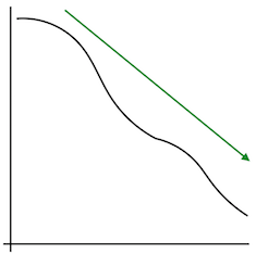
But, if the sweet spot is too narrow, we may miss it using an iterative approach:
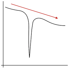
Or, we may hit a local minimum:
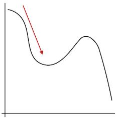
Stochastic Gradient Descent and other optimization techniques can help with these problems.
You can find more details about various optimization approaches in An Overview of Gradient Descent Optimization Algorithms.
It is sometimes useful to map a numeric relationship from one range to another.
For example, we might want to control the movement of a robotic arm with our finger such that a finger motion of 1cm in either direction along a specific axis will correspond to a 100cm motion in the same direction by the robotic arm.
Processing and other creative computing libraries provide the following function for this:
float map(float value, float istart, float istop, float ostart, float ostop)
{
      return ostart + ( ostop - ostart ) * ( ( value - istart ) / ( istop - istart ) );
}
where \(istart\) and \(istop\) represent the minimum and maximum values in the input range,
\(ostart\) and \(ostop\) represent the minimum and maximum values in the output range
and \(value\) represents a value within the input range that we wish to map to the output range.
For example:
map( 0.5, -1.0, 1.0, -100.0, 100.0 );Gives us:
\( \begin{align} output & = -100.0 + ( 100.0 - -100.0 ) * ( ( 0.5 - -1.0 ) / ( 1.0 - -1.0 ) ) \\ & = 50.0 \\ \end{align} \)
In computing the outputs of a neural network, it will be numerically convenient for the numeric domain of the output to be aligned with the numeric domain of the input.
By aligning the input and output domains, the derivative of the output with respect to the input can be expressed in terms of the output itself.
We use an activation function to produce this alignment.
Two commonly used activation functions are the sigmoid and tanh functions:
def sigmoid(x):
    return 1.0 / ( 1.0 + np.exp( -x ) )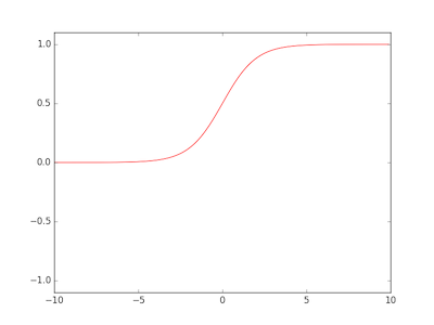
def tanh(x):
    return np.sinh( x ) / np.cosh( x )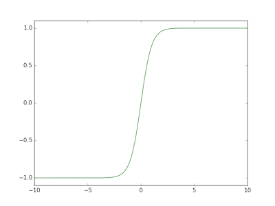
Notice that the sigmoid and tanh functions are very similar to one another.
The key difference is that the output domain of the sigmoid function is [ 0 .. 1 ] whereas output domain of the tanh function [ -1 .. 1 ].
One difficulty that can arise in supervised learning systems is the problem of overfitting in which the network tries to fit the training data so closely that it distorts the contour of the more general function that the training data is meant to exemplify.
Unsupervised learning systems create imitations of the patterns they've been trained on. However, they are learning the underlying probability of a given pattern within and with respect to the overall set of example patterns. Therefore, when the unsupervised system imitates a particular pattern, it does not produce an exact replica of it, but instead produces an imitation that accounts for similar patterns.
As a result, the pattern produced by an unsupervised system should contain the essential aspects of the pattern it is imitating, but smooths some of the individual quarks and noise contained in any specific training pattern.
By training a classifier on these smoothed or abstracted imitations rather than on the raw training samples, we can diminish overfitting.
There are many other amazing things you can do with unsupervised learning systems.
We'll take a closer look next week!
Assignment
Readings
Optional